| Block | Variables | What it describes | Members |
|---|---|---|---|
| participants | 6 | Who and what took part. Fixed once the collision is under way, though not in the longer run. | Type of collision, Car or light truck, Motorcycle or moped, Heavy vehicle, Bicycle, Vehicles involved |
| environment | 9 | The road and the conditions on it. What an engineer could change. | Road alignment, Road category, Weather, Road configuration, Lighting, Surroundings, Road surface, Location along road, Speed limit |
| temporal | 3 | When it happened. Partly reachable through enforcement and scheduling. | Time of day, Day of week, Month |
4 Which variables matter
4.1 A different question
Chapter 3 asked how well anything could predict severity, and found the limit low and lying in the data. A city adopting Vision Zero wants an answer to a different question: whether anything under its control affects how badly collisions turn out.
The two questions come apart here, and how they come apart is the substance of this chapter. The variables that predict are largely the ones nobody chooses, while the variables a city could change predict least.
Separating them means grouping the variables by what kind of thing they describe. Table 4.1 gives that grouping, declared once in the schema rather than assembled afresh for each analysis.
The geography block does not appear, because this analysis is restricted to one region and a variable with one value cannot separate anything. It exists in the schema so that a province-wide version of the same question has somewhere to put it.
ImportantWhat “outside anyone’s control” does and does not mean
Calling the participant variables uncontrollable is true only in a narrow sense.
Once two vehicles are converging, nobody chooses whether one of them is a bicycle. But over years a city chooses a great deal about how often bicycles and cars converge at all. Separated lanes, signal phases that hold turning traffic while people cross, and junctions designed so that a right-turning driver is not crossing a cycle track are exactly interventions in who meets whom, and the Montréal collisions in Chapter 5 turn on exactly such geometry.
This analysis cannot see any of that, because of what it conditions on. Every figure in this book is computed over collisions that occurred. Design that prevents an encounter removes a collision from the record rather than changing its severity, and a dataset of collisions has nothing to say about the ones that did not happen.
So the finding of this chapter is narrower than “road design does not matter”: given a collision has occurred, the recorded features of the road say little about how badly it turns out. Whether design changes how often collisions occur, and between whom, is a different question, answerable from different data, and Chapter 5 describes work that answers it.
4.2 What each block contributes
Write \(S(F)\) for the Matthews correlation of a model fitted using the feature set \(F\) and scored by cross-validation, with the folds, the preprocessing and the estimator held identical throughout. The estimator comes from the experiment specification, gradient-boosted trees; Chapter 3 established that the choice makes almost no difference, and any of the five families there would give the same picture.
Each block \(B\) then gets two figures.
\[\text{alone}(B) = S(B), \qquad \text{added}(B) = S(\text{all variables}) - S(\text{all variables except } B)\]
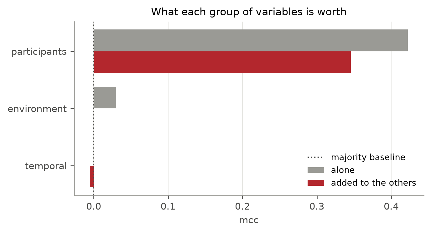
Alone is what the block achieves by itself, with everything else withheld: how much it would tell you if it were all you had.
Added is a difference of two correlations rather than a correlation. It fits on the full variable set, fits again with this block removed, and subtracts. A positive value means the block contributes something the others do not; zero means it contributes nothing new; and a negative value means the model does better without it.
The two figures can disagree, and where they do the disagreement tells you something. A block that scores well alone while adding nothing is carrying information the other blocks already carry. For deciding what to collect, the second figure is the relevant one.
| Block | Variables | MCC alone | MCC added | Balanced accuracy alone | Recall on serious, alone |
|---|---|---|---|---|---|
| majority baseline | 0 | 0.0000 | 0.3333 | 0.000 | |
| all features | 18 | 0.4118 | 0.4399 | 0.017 | |
| participants | 6 | 0.4223 | 0.3455 | 0.4363 | 0.000 |
| environment | 9 | 0.0299 | 0.0006 | 0.3354 | 0.000 |
| temporal | 3 | 0.0000 | -0.0049 | 0.3333 | 0.000 |
The pattern is not close. Knowing who was involved adds +0.3455 to the Matthews correlation. Knowing everything the SAAQ records about the road and the conditions on it adds +0.0006. The three time variables add -0.0049.
Taken alone, the environment block reaches 0.0299 against a baseline of 0.0000 for a rule that reads no variables at all.
Two features of that table deserve more than a passing mention.
A negative contribution is possible, and one block has one. Where removing a block improves the score, the block was contributing noise that the model fitted and that did not survive to the validation fold. A contribution below zero therefore says more than a contribution of zero would.
The participant block alone scores 0.4223, and the full variable set scores 0.4118. The best model available on this data uses six variables and would be no better, on this measure, for having the other twelve.
There is one qualification, and it points the other way. Read the recall column of Table 4.3 rather than the correlation. Recall on serious collisions rises as blocks are added, from nothing at all to a couple of percent. The extra variables do let the model occasionally name the severe class and occasionally be right about it, at a net cost in overall agreement. Both figures are true, and neither is a working model: a couple of percent is not a detector.
4.4 The variables an engineer could change
An ablation reports a number, and a number on its own invites the suspicion that something has been done wrong, so it helps to see why this one comes out as it does.
Table 4.4 breaks the outcome down by each environment variable in turn. If any of them mattered, its values would show visibly different outcome distributions.
The rate of serious injury for a given value of a variable is the number of collisions carrying that value whose outcome was serious or fatal, divided by the number carrying that value. Records where the variable was left blank are excluded from both. For scale, the rate across all Montréal collisions is 0.0086.
| Variable | Values shown | Lowest rate of serious injury | Highest rate of serious injury | Spread |
|---|---|---|---|---|
| Road alignment | 2 | 0.0087 | 0.0132 | 0.0046 |
| Road category | 2 | 0.0036 | 0.0095 | 0.0059 |
| Weather | 10 | 0.0025 | 0.0162 | 0.0137 |
| Road configuration | 4 | 0.0054 | 0.0114 | 0.0060 |
| Lighting | 4 | 0.0073 | 0.0233 | 0.0160 |
| Surroundings | 6 | 0.0073 | 0.0161 | 0.0087 |
| Road surface | 8 | 0.0033 | 0.0111 | 0.0078 |
| Location along road | 6 | 0.0033 | 0.0141 | 0.0109 |
| Speed limit | 6 | 0.0036 | 0.0128 | 0.0092 |
These spreads are not zero. The widest of them is Lighting, whose rate of serious injury runs from 0.73% to 2.33% across its values. Against an overall rate of 0.86% that is a difference of several times over, not a rounding error.
So how does a variable show a tenfold difference in outcome rate and then contribute +0.0006 to a model?
Because the two questions are different. A breakdown by one variable at a time shows every association, including associations that belong to something else. Collisions in the dark involve a different mix of road users, at different speeds, in different places. The lighting variable is standing in for all of that. Once the model already knows who was involved, the lighting column has little left to tell it, and what remains after everything else has spoken is what the ablation measures.
This is the ordinary difference between a marginal and a conditional association, and it explains why a table of one-variable breakdowns makes a poor guide to what a city should collect.
4.4.1 A variable that is not what it is filed under
The lighting variable illustrates this well enough to follow up.
Read its definition rather than its name. It takes four values, and the first two are daytime: full daylight, and the half-light around dawn and dusk. The second two are night, distinguished by whether the road had working lighting installed.
| Value | Definition |
|---|---|
| Clear day | Day and clarity. Day: Period between half an hour before sunrise and half an hour after sunset. Clarity: Refers to the period between sunrise and sunset. |
| Dawn/dusk | Day and half darkness. Day: Period between half an hour before sunrise and half an hour after sunset. Half-darkness: Refers to the period between night and sunrise and the period between sunset and night. |
| Lit path | Night and lit path. Night: Period between half an hour after sunset and one half an hour before getting up. Illuminated path: Path along which lighting equipment is installed which was operating at the time of the accident. |
| Unlit path | Night and unlit path. Night: Period between half an hour after sunset and one half an hour before getting up. Unlit path: Path along which, in the immediate area of the accident, no lighting equipment is installed or the equipment in place was not functioning. |
So most of what this variable encodes is the time of day. Only one contrast within it, the third value against the fourth, describes anything a city installs and maintains.
| LIGHT | Clear day | Dawn/dusk | Lit path | Unlit path |
|---|---|---|---|---|
| HOUR | ||||
| 00:00-04:00 | 0.035 | 0.005 | 0.939 | 0.021 |
| 04:00-08:00 | 0.645 | 0.101 | 0.247 | 0.006 |
| 08:00-12:00 | 0.974 | 0.012 | 0.013 | 0.001 |
| 12:00-16:00 | 0.968 | 0.022 | 0.009 | 0.001 |
| 16:00-20:00 | 0.586 | 0.119 | 0.290 | 0.005 |
| 20:00-24:00 | 0.056 | 0.041 | 0.884 | 0.019 |
Each row covers the collisions in one four-hour band and divides them among the four lighting states, so the entries in a row sum to one. The figure in row \(i\) and column \(j\) is the share of collisions in band \(i\) that were recorded with lighting state \(j\).
The correspondence is nearly complete. In 4 of the six time bands, one of the two states accounts for more than eighty-five percent of collisions: the middle of the day is daylight and the middle of the night is not, which is not a finding about roads.
The two bands that are genuinely mixed are the ones straddling sunrise and sunset. There the lighting variable does carry something the hour does not, because six in the morning is dark in December and bright in June. What it adds over the time variables, in other words, is mostly a seasonal correction to them.
This matters for reading Table 4.2. The block called environment contains a variable that is largely a time variable, and the block called temporal therefore has less left to contribute than its name suggests. Blocks are a convenience for asking a question, not a property of the data, and no assignment of these twenty-five variables into four groups is going to be clean.
It also suggests a better question. Rather than asking what lighting contributes in general, ask what it contributes where a city could change it: among collisions that happened at night, does a lit road differ from an unlit one?
| At night, the road was | Collisions | No injury | Minor injury | Serious or fatal |
|---|---|---|---|---|
| Lit path | 84,695 | 0.7927 | 0.1944 | 0.0129 |
| Unlit path | 1,804 | 0.8226 | 0.1541 | 0.0233 |
The unlit column has a rate of serious injury 1.8 times that of the lit one. Taken at face value the difference is substantial, and it does not come from a small sample: there are 1,804 collisions in that column.
It should not be taken at face value, for two reasons.
The first is the shape of the difference. If darkness were the mechanism, one would expect outcomes to shift toward the worse across the board. They do not. The unlit column has a higher share of collisions causing no injury at all as well as a higher share causing serious injury, and a lower share of the minor injuries in between. A pattern like that points to a different mix of collisions rather than a shift in severity. Fewer people on foot and on bicycles, who generate most of the minor injuries, together with higher speeds, which generate the serious ones, would produce exactly this.
The second is that unlit roads are not a random sample of roads. They are 2.1% of night-time collisions in Montréal, and the places within a city that have no street lighting are systematically the peripheral, faster and emptier ones. Comparing them with lit roads compares two different kinds of place, and the extract records the difference between those places only through the same coarse variables that Table 4.4 already showed carry little.
So this comparison does not estimate what installing street lighting would achieve. It reports that collisions on unlit roads at night differ from collisions on lit roads at night, which is true, and consistent with several explanations, of which lighting is one.
For comparison, Table 4.8 gives the same breakdown for the variables describing who was involved.
| Variable | Values shown | Lowest rate of serious injury | Highest rate of serious injury | Spread |
|---|---|---|---|---|
| Type of collision | 6 | 0.0034 | 0.0787 | 0.0753 |
| Car or light truck | 2 | 0.0077 | 0.0218 | 0.0141 |
| Motorcycle or moped | 2 | 0.0079 | 0.0484 | 0.0405 |
| Heavy vehicle | 2 | 0.0086 | 0.0086 | 0.0000 |
| Bicycle | 2 | 0.0077 | 0.0360 | 0.0283 |
| Vehicles involved | 3 | 0.0043 | 0.0278 | 0.0234 |
The contrast is the point. The widest spread among the participant variables is Type of collision, running from 0.34% to 7.87%, which is 4.7 times the widest spread among the variables describing the road.
One row in Table 4.8 deserves a note of its own. The heavy vehicle indicator shows no difference at all: collisions involving a heavy vehicle in Montréal are as likely to produce a serious injury as those that do not. The intuition that says otherwise comes from highway collisions at speed, and a dense urban network is a different setting, where most heavy vehicle involvement is low-speed manoeuvring.
4.5 The same question without a model
Everything above rests on fitting something. A sceptic may reasonably ask how much of the answer belongs to the data and how much to the estimator, the folds, or the choice of metric.
The question can be put without fitting anything at all.
Take two collisions that agree on every recorded variable outside one block, so that whatever separates them lies inside it. How often do they share an outcome? If the block carries nothing, agreeing outside it means agreeing on everything that matters, and such pairs should usually turn out alike. If the block carries a great deal, differing within it should pull them apart.
| Block | Variables | Pairs | Share alike | Same size, at random | Difference |
|---|---|---|---|---|---|
| participants | 6 | 2,742,140 | 0.5428 | 0.6480 | -0.1052 |
| temporal | 3 | 64,699,700 | 0.6723 | 0.6623 | 0.0100 |
| environment | 9 | 175,689,082 | 0.7229 | 0.6646 | 0.0583 |
NoteWhy the comparison is against random blocks
The obvious reference, records identical throughout, cannot be used. Agreement over a partition weights each group by the pairs it contains, so refining a partition destroys its large groups and the weight does not redistribute evenly. A finer partition can therefore show lower agreement than a coarser one, and records identical throughout are not an upper bound on anything.
The same objection rules out comparing blocks with each other directly, since agreeing outside a small block is a stronger condition than agreeing outside a large one. The control here is a block of the same size drawn at random, which faces identical granularity, and the difference between them measures what the block’s membership buys.
Two rows repay a closer look.
Pairs differing only in who was involved share an outcome 0.5428 of the time, against 0.6398 for two collisions picked at random from the whole dataset. Holding the road, the conditions and the time of day all fixed, and letting only the participants vary, leaves two collisions less alike than if nothing had been held fixed at all. A variable that determines the outcome looks exactly like this from this angle.
Pairs differing only in the road and the conditions on it run +0.0583 above a random block of the same size. So those variables are not merely uninformative in the sense of adding nothing to a model. They carry less than an arbitrary handful of variables would.
No model was fitted to produce that table, no metric was chosen, and no hyperparameter was set, and the result agrees with Table 4.2, which is why it was computed.
4.5.1 One variable at a time
The same construction narrows to a single variable: pairs agreeing on all seventeen others and differing in exactly one.
Take a collision that was serious and another that agrees with it on all seventeen remaining variables, differing only in the one named. How likely is that second collision to have been serious too?
Write \(\pi\) for the share of all records that were serious. For a variable \(v\), let \(q(v)\) be the share of such neighbours that were serious. The lift is
\[\mathrm{lift}(v) = \frac{q(v)}{\pi} .\]
A lift of one would mean the neighbour is no more likely to be serious than a collision drawn at random; larger values mean the pair resembles itself in outcome as well as in circumstance.
| Variable | Pairs | Lift | Share of the reference |
|---|---|---|---|
| Location along road | 5,406 | 1.812 | 0.73 |
| Speed limit | 6,430 | 2.031 | 0.82 |
| Time of day | 10,953 | 2.068 | 0.84 |
| Month | 41,892 | 2.363 | 0.96 |
| Surroundings | 6,161 | 2.882 | 1.17 |
The reference is 2.469, the lift among records identical throughout. Changing a variable that carries nothing leaves the enrichment intact, so an inert variable sits at the reference; one that carries something pulls it below.
Only a handful of variables appear, because pairs differing in exactly one of eighteen are rare and most variables have too few for the ratio to mean anything. The participant variables are absent for that reason rather than because they do nothing, which is a limitation of this view and not a finding.
Within what is shown, location along the road and the posted speed limit are the two that move the outcome most. Both belong to the block that Table 4.2 found contributes almost nothing. There is no contradiction. This table asks what a variable does with every other held fixed; the ablation asks what it adds once every other is already known. A variable that shifts the outcome on its own can still add nothing to a model that already knows the rest.
4.6 Conditioning the obvious away
The dominance of the participant variables is not a discovery. Pedestrians and cyclists get hurt when vehicles strike them, which nobody disputes and which no road authority can design around by wishing there were fewer pedestrians.
A more useful question is what happens once that is taken as given. Among collisions that struck a pedestrian, what distinguishes the serious ones from the rest?
That subproblem is better posed in two ways. The class balance is far less extreme, so the scarce class is no longer buried, and the participant variables that dominate the general problem are largely constant within it and cannot do the work.
| Outcome | All Montréal collisions | Pedestrian collisions only |
|---|---|---|
| Material damage only | 76.8% | 14.3% |
| At least one minor injury | 22.2% | 77.9% |
| Serious injury or fatality | 1.0% | 7.8% |
| Block | Variables | MCC alone | MCC added | Recall on serious, alone |
|---|---|---|---|---|
| majority baseline | 0 | 0.0000 | 0.0000 | |
| all features | 17 | 0.1102 | 0.0421 | |
| participants | 5 | 0.0960 | 0.0910 | 0.0066 |
| environment | 9 | 0.0072 | 0.0034 | 0.0133 |
| temporal | 3 | 0.0013 | -0.0096 | 0.0011 |
Everything is smaller here, as it should be. Conditioning on a pedestrian being struck removes the part of the problem that was easy, and what remains is the part nobody knew the answer to. The full variable set reaches 0.1102, against roughly four tenths in the general problem.
The ordering, though, is unchanged. Who else was involved adds +0.0910. Everything about the road adds +0.0034. The time variables again subtract.
The participant variables here are no longer the type of collision, which is constant by construction, but whether the vehicle that struck the pedestrian was a car, a truck, a motorcycle, or one of several. Their continued dominance carries a blunt summary: what hit you matters more than where you were standing.
There is one respect in which the environment does better. Relative to what the participant variables contribute, it accounts for 3.7% here against 0.2% in the general problem. That change runs in the direction one would expect, since speed limit and lighting have a plausible mechanism for a person on foot that they do not have for two cars meeting at a junction.
Little rests on it. This subproblem has a few thousand records rather than a few hundred thousand, and a contribution of a few thousandths of a correlation coefficient at that sample size is not distinguishable from nothing. The most that can be said is that the environment variables are not measurably more useful here, only less overwhelmed.
4.7 Night, and what cannot be said about it
Suppose the time variables do carry more weight in the pedestrian problem than in the general one, and that lighting is among the variables that move the outcome. The obvious reading is that pedestrians struck in the dark are hurt worse because drivers cannot see them, and the obvious recommendation is more street lighting.
That reading may be correct. This data cannot establish it, for reasons that generalise well beyond this variable.
Several explanations fit equally well.
- Drivers see less in the dark, so collisions happen at higher effective speed and with less braking.
- Traffic is lighter at night, so drivers travel faster on the same roads.
- More drivers and more pedestrians have been drinking in the evening.
- The people out walking at two in the morning are not the same people out walking at two in the afternoon, in age, in sobriety, and in where they are walking.
- Emergency response and hospital staffing differ overnight, which affects how an injury is graded and how it resolves.
The extract records none of the quantities that would separate these. There is no speed travelled, no alcohol measurement, no traffic volume, no age, no time to treatment. Every one of the explanations above shows up in this data as the same thing: a collision at night that hurt somebody.
And even if darkness were the whole story, the intervention does not follow cleanly. No amount of street lighting turns night into day. The question a road authority faces is not whether darkness is worse but how much a given lighting improvement would buy, and that is a question about magnitudes on a scale this data does not measure.
ImportantThe shape of the problem
The variables that predict are the ones nobody chooses. The variables anyone could change barely predict. And where an actionable variable does appear to matter, the data cannot distinguish its effect from several confounders it never recorded.
Each of those three is a limitation. Together they are a finding about what administrative collision records can support, and it applies well beyond Quebec.
4.8 What this means for a road safety programme
None of this says that road design has no effect on how badly collisions turn out. That would be a strange conclusion, and the data does not support it.
The two claims are easily confused. Table 4.4 showed that the rate of serious injury does vary across road conditions, by several times over in the case of lighting. What the ablation adds is that this variation is not information the road variables contribute; it is information already carried by who was involved and where they were. The association holds, and adds nothing once the rest of the form has been read.
What the data supports is narrower and, for anyone planning to use records like these, more useful. Collision reports as collected here are not an instrument capable of detecting the effect of road design on severity. The variables are too coarse, the most relevant ones are missing, and the ones that are present are dominated by a fact about who was involved that no design can alter.
An analysis of this data that reported which road features are dangerous would not be reporting a discovery. It would be reporting the noise left over after the participant variables had taken everything there was.
Chapter 5 sets out what would be needed instead.