| Collisions | No injury | Minor injury | Serious or fatal | Commonest outcome's share |
|---|---|---|---|---|
| 132 | 83 | 48 | 1 | 0.629 |
| 132 | 84 | 47 | 1 | 0.636 |
| 115 | 72 | 43 | 0 | 0.626 |
3 How well could anything do?
Everything in this chapter concerns the 235,925 Montréal records available for fitting, described at the end of Chapter 1, with the 18 features that survive the exclusions in Chapter 2. The held-out records are not touched.
The question is not whether the model built in the usual way performs well. The question is whether any method could, which is a different question with a different kind of answer. It can be settled without building a good model, because it does not depend on how good the model is.
3.1 Collisions recorded identically
Start with something concrete.
Group the records so that every collision in a group has exactly the same value for every one of the 18 recorded variables: the same weather, the same road surface, the same lighting, the same road configuration, the same hour, the same month, the same vehicle types, everything. Call each such group a cell.
Table 3.1 shows the three largest cells in which the outcomes disagree.
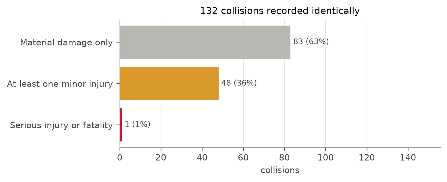
Now consider what a classifier does with that cell. It reads the recorded variables and returns an answer. Every collision in the cell presents it with the same input, so it returns the same answer for all of them. It has no choice about this: identical inputs, identical output.
The most accurate thing it can do on that cell is answer with whichever outcome is commonest there. Nothing does better on the proportion correct, though a method chasing something else may well prefer a different answer, and Section 3.3 takes that up. That holds for a lookup table, a boosted ensemble, a neural network of any size, and a person with an intuition, because it follows from the inputs being identical rather than from anything about the method.
ImportantThe whole argument, in one sentence
A method has to give the same answer to the same input, so within a cell it cannot be right more often than the rule that always answers with that cell’s commonest outcome.
Call that the cell-majority rule, a name that recurs throughout the chapter. Nothing about it is a model: it holds no parameters, is fitted to nothing, and looks up what happened last time to collisions recorded the same way.
Which means it cannot generalise at all. Faced with a combination of circumstances that has never occurred, it has nothing to look up and no answer to give. The limitation is a serious one and Section 3.4.2 measures it; for the moment the rule serves only to establish what could be achieved on collisions that do have counterparts on record.
Table 3.1 supports two readings, and the chapter needs both of them kept apart.
The pessimistic one is that these collisions cannot be told apart. Whatever distinguished the one that hurt somebody from the ones that did not, it is not written on the form.
The optimistic one is that the cell is not the same as the dataset. If the outcome shares within it differ from the overall shares, then knowing where a collision falls does tell you something, just not enough to name the outcome. Chapter 5 returns to that, since it is the most the data will support.
3.2 How often do identical collisions disagree?
Do that for every cell, count the records that match their own cell’s commonest outcome, and divide by the number of records counted. Table 3.3 reports the result.
WarningWhat this table is for, and what it is not for
The figure it produces is a genuine upper bound on accuracy, and a nearly useless one. Read the first row and it says that no method exceeds about ninety-three percent, while a rule that ignores every variable and always answers “no injury” reaches about seventy-seven. A bound sixteen points above the trivial answer forbids very little.
Two things are wrong with it, and both are instructive. Most cells hold one record and a cell of one always agrees with itself, so the bound is inflated by cells that could not have been wrong. And accuracy was the wrong target from the start, for reasons Section 3.3 sets out.
The table is here for what its last column shows rather than for the bound in its third. Read down that column. The statements this book relies on come later: Table 3.5 for accuracy and for balanced accuracy, and Table 3.6 for a statement that needs no metric at all.
| Cells of at least | Distinct cells | Records covered | Share of records | Accuracy bound | Share in mixed cells |
|---|---|---|---|---|---|
| 1 | 147,866 | 235,925 | 100.0% | 0.9205 | 0.280 |
| 2 | 27,808 | 115,867 | 49.1% | 0.8382 | 0.570 |
| 5 | 5,861 | 61,746 | 26.2% | 0.8132 | 0.778 |
| 10 | 1,945 | 36,901 | 15.6% | 0.7972 | 0.879 |
| 20 | 554 | 18,677 | 7.9% | 0.7765 | 0.943 |
| 50 | 64 | 4,719 | 2.0% | 0.6940 | 0.987 |
Each row keeps only the cells at or above the stated size and reports on the records in them, so the rows describe progressively smaller parts of the data, made up of the collisions whose exact circumstances recur most often. Two of the columns need defining.
Accuracy bound is the share of covered records whose outcome matches their own cell’s commonest outcome. No method can achieve better accuracy on those records.
Share in mixed cells is the fraction of covered records living in a cell where more than one outcome occurs. In a cell with only one outcome, the cell-majority rule names that outcome and is right about every record in it, so those records raise the bound without ever constraining it. Only mixed cells force any error. This column therefore says how much of each row rests on cells that could have brought the bound down.
The cut-offs are a selection rather than a complete list. Every integer from one upwards gives a row, and the six shown are enough to see the shape.
3.2.1 A small example, worked by hand
The same calculation on a dataset small enough to check by hand makes Table 3.3 easier to read. Suppose there are ten collisions falling into five cells:
| Cell | Records | Outcomes | Commonest outcome occurs |
|---|---|---|---|
| A | 4 | no injury, no injury, no injury, minor injury | 3 |
| B | 3 | no injury, no injury, no injury | 3 |
| C | 1 | minor injury | 1 |
| D | 1 | no injury | 1 |
| E | 1 | serious | 1 |
| Cells of at least | Distinct cells | Records covered | Share of records | Accuracy bound | Share in mixed cells |
|---|---|---|---|---|---|
| 1 | 5 | 10 | 100% | 0.9000 | 0.4000 |
| 2 | 2 | 7 | 70% | 0.8571 | 0.5714 |
| 3 | 2 | 7 | 70% | 0.8571 | 0.5714 |
| 4 | 1 | 4 | 40% | 0.7500 | 1.0000 |
Every figure in that table can be checked directly.
The first row counts all five cells and all ten records. Its bound is the sum of the final column of the list above, divided by ten: \((3+3+1+1+1)/10 = 0.9\). Only cell A is mixed, and it holds four records, so four in ten of the covered records are in a mixed cell.
The second row ignores cells C, D and E, leaving A and B with seven of the ten records between them. The bound is now \((3+3)/7 \approx 0.857\), and four of those seven records are in a mixed cell.
The third row is identical to the second, because no cell holds exactly two records: raising the cut-off from two to three excludes nothing. A row changes only when the cut-off passes an actual cell size, which here means at 2 and at 4. On the full dataset cells occur at every size, so consecutive cut-offs differ and no rows coincide.
The fourth row keeps only cell A. The bound is \(3/4 = 0.75\) over four records, and every one of them is in a mixed cell.
Three things follow, and all three carry over to the real data.
The rows are nested, not a partition. Every record in the second row is also in the first. Adding the rows together, or multiplying a cut-off by a cell count, does not give the size of the dataset: for this example that arithmetic gives thirteen, and there are ten records.
The bound is not the share of the commonest outcome overall. Seven of these ten collisions caused no injury, so a rule that always answered “no injury” would score 0.7. The bound in the first row is 0.9, because the cell-majority rule answers differently in different cells. The gap between those two numbers measures what the variables buy you.
Singletons push the first row up. Cells C, D and E each contribute a perfect score while demonstrating nothing, which is why the bound falls once they are excluded. The data does not become harder to predict further down the table. The earlier rows were counting cells that could not have been wrong.
3.2.2 Reading the real table
Read across the rows of Table 3.3 and the bound appears to fall as the cut-off rises. The bound is not falling: each row describes a different population, and the ones further down cover fewer records, all of them from combinations that occur many times over. The reason to raise the cut-off is that the first row is inflated by cells too small to say anything.
The last column carries the finding. In the first row, roughly three quarters of records sit in a cell with a single outcome, which sounds encouraging until one notices that most of those cells hold one record. Further down, where cells are large enough to say anything at all, almost every record still counted sits in a cell whose outcomes disagree.
The rest of the chapter rests on that claim, which is not a claim about accuracy. It says the recorded variables do not determine the outcome: take collisions that agree on all eighteen and occur often enough to be counted, and they still turn out differently from each other. How much that costs, and in which currency, is what the following sections measure.
WarningWhy the first row proves little
A cell containing one record always agrees with itself. Its commonest outcome is the only outcome it has, so it contributes a perfect score to the bound while demonstrating nothing.
With 18 variables most cells are that small. The first row of Table 3.3 is therefore mostly measuring how many distinct combinations exist, not how predictable anything is. The demonstration is in Section 3.9: shuffle the outcomes at random, so that nothing is predictable by construction, and that first number barely moves.
3.3 What if accuracy is the wrong target?
Everything so far has measured accuracy, and accuracy is close to the worst thing to measure here. Nobody cares about the proportion correct when only one collision in a hundred matters.
The cell-majority rule maximises the proportion correct, which is why it appeared first. On data where four collisions in five caused no injury it will answer “no injury” in almost every cell, and its recall on serious collisions will be close to zero. It scores well by declining to look for the thing the analysis is about.
So the question is whether the argument survives a change of target. It does, and the reason is the part that never mentioned accuracy:
ImportantWhat the cells fix, and what they leave open
Because every record in a cell presents the same input, any method answers a whole cell the same way. So a method is entirely described, as far as these variables are concerned, by which outcome it names in each cell.
There are finitely many such methods, and each produces one confusion matrix and hence one value for whatever one chooses to measure. Collect those values and the result is a fixed set of attainable scores, determined by the cells’ outcome distributions and by nothing else.
Choosing a metric picks a point in that set. It does not move the set, and it does not move the set’s outer edge: the methods that cannot be improved in one respect without giving something up in another. That edge is what the rest of this section is about.
Table 3.5 gives two rules on the same cells. The first is the cell-majority rule. The second answers with whichever outcome is most over-represented in the cell, and that phrase should be made exact.
Write \(x_k\) for the share of class \(k\) across the whole dataset and \(y_k\) for its share within some cell. The second rule names the class \(j\) maximising the ratio \(y_j / x_j\). Where the cell-majority rule asks which outcome is commonest here, this asks which outcome is commonest here compared with how common it is generally.
That ratio is not an arbitrary choice. The mean of the per-class recalls, which is balanced accuracy, is \(\frac{1}{M}\sum_k C_k / N_k\), where \(N_k\) is the number of records of class \(k\) and \(C_k\) the number the rule gets right. Write \(n_j\) for the number of records of class \(j\) in some particular cell. If that cell is assigned class \(j\) it adds \(n_j\) to \(C_j\) and nothing to any other \(C_k\), so each cell independently wants the \(j\) maximising \(n_j / N_j\). Since \(n_j\) is the cell’s size times \(y_j\), and \(N_j\) is the dataset’s size times \(x_j\), that is the same as maximising \(y_j / x_j\).
An example makes the difference concrete. Suppose the three outcomes occur overall in the proportions \(x = (0.77, 0.19, 0.04)\), and consider a cell in which they occur as \(y = (0.60, 0.30, 0.10)\). The ratios are
\[\frac{0.60}{0.77} = 0.78, \qquad \frac{0.30}{0.19} = 1.57, \qquad \frac{0.10}{0.04} = 2.40 .\]
The cell-majority rule names the first outcome, which occurs in three collisions out of five there. The second rule names the third outcome, which occurs in one out of ten, because one in ten is more than twice its usual rate. The first rule will be right more often. The second will find serious collisions that the first never looks for.
| Quantity | Commonest outcome | Most over-represented outcome |
|---|---|---|
| Accuracy | 0.7778 | 0.6577 |
| Balanced accuracy | 0.4150 | 0.4519 |
| Recall, Material damage only | 0.9215 | 0.6904 |
| Recall, At least one minor injury | 0.3099 | 0.5625 |
| Recall, Serious injury or fatality | 0.0137 | 0.1027 |
Each column is a ceiling for the thing its rule maximises, and neither is a ceiling for anything else. A rule tuned for some third objective would beat both columns on that objective and lose to both on theirs, while still landing inside the same fixed set.
For scale: always answering “material damage only”, using no variables at all, achieves an accuracy of 0.7684 on the same records. Compare that with the first column.
What the figures speak for. They are computed over the 45.8% of validation records whose exact combination of variables appeared at least once in the training part. The rest are combinations never seen before, about which any rule built from cells has nothing to say at all.
That share is itself a finding, and a discouraging one. Even with 188,740 records to learn from, a large fraction of new collisions are unlike anything on record.
3.4 The bound that does not need a metric
The limit can be stated without choosing an objective at all, and this is the strongest form of the argument in the chapter.
Change the question from classification to flagging. Suppose a road authority wants to mark some collisions as the ones likely to be serious, and can accept being wrong sometimes. How well could that be done?
The question has become a two-way one rather than a three-way one, and the reduction is deliberate. Every collision receives one of two verdicts, flagged or not flagged, where not flagged means predicted not serious and puts material damage and minor injury together. Precision and recall then have their ordinary binary meanings for the flagged class: precision is the share of flagged collisions that were serious, recall is the share of serious collisions that were flagged.
Collapsing three outcomes into two is what makes the rest of this section possible. With three classes a rule must choose one of them for each cell, and describing everything attainable means describing a large and awkward set. With one class singled out, a rule is nothing more than a set of cells to flag, the sensible ones are nested inside each other, and the whole attainable set is a single sweep that can be written down.
Since every record in a cell looks identical, a rule flags either all of a cell or none of it. A rule is therefore fully described by which cells it flags, and the sensible strategy is clear: to flag a given number of collisions and be right as often as possible, flag the cells where serious injury was commonest in the past. Start with the worst cell, then add the next worst, and so on.
Each stopping point along that sweep is one rule, and Table 3.6 lists them.
| Flag cells whose past rate is at least | Collisions flagged | Of those, actually serious | Of all serious ones, share flagged |
|---|---|---|---|
| 1.0000 | 51 | 0.0392 | 0.0043 |
| 0.5000 | 91 | 0.0440 | 0.0087 |
| 0.2500 | 164 | 0.0366 | 0.0130 |
| 0.1667 | 243 | 0.0288 | 0.0152 |
| 0.1250 | 277 | 0.0253 | 0.0152 |
| 0.0952 | 322 | 0.0217 | 0.0152 |
| 0.0769 | 382 | 0.0209 | 0.0173 |
| 0.0625 | 433 | 0.0231 | 0.0216 |
| 0.0526 | 483 | 0.0207 | 0.0216 |
| 0.0455 | 517 | 0.0271 | 0.0303 |
| 0.0385 | 535 | 0.0262 | 0.0303 |
| 0.0333 | 560 | 0.0250 | 0.0303 |
| 0.0213 | 595 | 0.0252 | 0.0325 |
| 0.0000 | 21,599 | 0.0068 | 0.3160 |
Every row is a complete rule, not a description of one cell. Given a held-out collision, look up its cell’s past rate, the share of that cell’s training records that were serious. If the rate is at or above the row’s stated figure, flag the collision; otherwise leave it. That yields a verdict for every held-out record, and the third and fourth columns are the ordinary precision and recall of those verdicts, over the whole held-out set rather than within any cell.
The first row is the most selective rule available and it gives the ceiling on precision, for a reason that takes one line. The precision of any rule is the number of serious collisions among the flagged records divided by the number flagged, which is an average of the flagged cells’ rates. An average cannot exceed its largest term. So no method can achieve a precision higher than the share of serious collisions in the single worst cell, however it is built, tuned or scored.
The last row is the least selective rule available: flag every cell the rule has ever seen. Precision falls to the rate of serious injury among those records, which is close to the overall rate.
Recall, though, does not reach one. A cell that never appeared in training has no past rate, so the rule has nothing to look up and flags nothing. Those collisions are missed whatever the threshold.
So the recall of any rule built from cells is capped at 0.3160, the share of held-out serious collisions whose exact combination had been seen before. Flagging everything it recognises still leaves the rest, and no threshold reaches them.
Set that figure against the one from the previous section. 45.8% of held-out collisions fall in a cell that appeared during training. Among the serious ones, 31.6% do.
Serious collisions are therefore markedly less likely than average to resemble anything on record, which follows from their being rare: an unusual combination of circumstances is by definition one that seldom recurs. The two effects compound. The class this analysis exists to study is both the scarcest and the one the data has least precedent for, and the second is not merely a restatement of the first.
Everything a cell-based method can do for this class lies along that sweep, and where it lies is fixed by the data. Choosing a metric picks a row. It cannot produce a row that is not there, and it cannot reach past the last one.
3.4.1 Why this constrains the three-class models too
Nothing above requires anyone to build a binary classifier, and the models elsewhere in this book are not binary.
Take any classifier over the three outcomes and read its verdicts as flags: where it predicts serious, treat the collision as flagged; where it predicts anything else, treat it as not flagged.
Its precision and recall on the serious class are then not merely bounded by the binary quantities defined above, they are equal to them. Both are per-class figures, and both count the same things: the collisions predicted serious form the flagged set, and the collisions both predicted and actually serious form the numerator of each. Neither quantity ever inspects how the remaining predictions were divided between material damage and minor injury, so the further decision a three-class classifier makes has no bearing on either.
The classifier reads only the recorded variables, so it answers every record in a cell the same way, and the flagging rule induced from it flags whole cells. It is therefore one of the rules the sweep already accounts for, and its precision and recall on the serious class name a point in Table 3.6. The sweep bounds every model in this book, not merely the rules used to construct it.
NoteWhy this needs no metric
Accuracy, balanced accuracy and every weighted combination of per-class scores are functions of a confusion matrix. A rule that flags a set of cells determines its confusion matrix, so it determines every such score at once.
The table above lists the confusion matrices available. Any metric one might prefer is a way of ranking those rows, and no ranking creates a row. Hence this bound survives the objection Section 3.3 raises, and hence Appendix B reports no weighted aggregate of its own.
3.4.2 How far does resemblance carry?
A fair objection to the previous section is that a model does not need an exact match. Faced with a combination of circumstances it has never seen, it borrows from combinations it has seen that are similar, and no classifier would be much use if it could not.
That borrowing rests on an assumption. Records close together in feature space are supposed to have similar outcomes, and where that holds a model has something to generalise along. The assumption is testable here, because the variables are categorical and closeness has an exact meaning: two collisions are at Hamming distance \(d\) when they differ on \(d\) of the recorded variables and agree on the rest. Distance zero is the cell.
Table 3.7 asks whether a collision’s near neighbours are more likely to be serious than a collision picked at random.
| Variables differing | Neighbour pairs | Share of neighbours serious | Ratio to the base rate | Counted |
|---|---|---|---|---|
| 1 | 90,047 | 0.02170 | 2.21 | exactly |
| 2 | 663,792 | 0.01795 | 1.83 | exactly |
| 3 | 11,091 | 0.01515 | 1.55 | sampled |
| 4 | 35,810 | 0.01329 | 1.36 | sampled |
| 5 | 87,974 | 0.01237 | 1.26 | sampled |
| 6 | 174,072 | 0.01044 | 1.07 | sampled |
| 7 | 275,914 | 0.00954 | 0.97 | sampled |
| 8 | 354,542 | 0.00918 | 0.94 | sampled |
| 9 | 369,440 | 0.00914 | 0.93 | sampled |
| 10 | 311,896 | 0.00930 | 0.95 | sampled |
| 11 | 210,206 | 0.00996 | 1.02 | sampled |
| 12 | 109,534 | 0.00997 | 1.02 | sampled |
| 13 | 42,369 | 0.01190 | 1.21 | sampled |
| 14 | 11,844 | 0.01393 | 1.42 | sampled |
The fourth column is the third divided by the share of all records that were serious, which is 0.00980. Read it as a multiple rather than a percentage: two means a neighbour is twice as likely to be serious as a collision drawn at random.
The last column matters too. Distances of two or less are counted exhaustively, by grouping on every choice of variables to ignore. Beyond that the pairs are sampled, which is adequate because two collisions drawn at random from 18 variables are almost never close: the space is sparse enough that most randomly chosen pairs differ on most fields. Rows are shown only where the base rate alone would produce a hundred neighbours or more, since a ratio computed from a handful of pairs is noise.
NoteWhat the ratio would look like if the features carried local structure
Run the same measure on constructed data where a rare outcome depends on two of ten variables and it returns a ratio of about four at the closest distances, falling below one at the furthest. That figure is measured rather than derived, and it would change with the strength of the dependence; what matters is that it is far from one and that it decays.
On constructed data where the outcome is independent of every variable, the ratio stays within a few percent of one at every distance.
Both are in the repository as tests, since a measure that cannot tell those two cases apart has nothing to report.
The ratio does fall away, which runs against what the rest of the chapter might lead one to expect and so needs stating clearly. Collisions differing in a single recorded variable are about twice as likely to share a serious outcome as a collision picked at random. The elevation shrinks with each further variable that differs and reaches chance at around six or seven. There is local structure here, and a model does have something to generalise along.
Two qualifications keep that from being good news.
The first is the size of the effect. Doubling a rate of one percent gives a rate of two percent. A collision’s closest neighbours are still, some ninety-eight times in a hundred, not serious. The structure is real and it is the same real-but-small quantity the rest of this chapter measures, arriving by another route.
The second is the far end of the table. The ratio does not settle at chance; it turns and climbs again among pairs differing on thirteen or fourteen variables. Collisions that are almost entirely unalike are somewhat more likely to share a serious outcome than collisions that are moderately unalike.
That shape is what one would see if serious collisions sat in several small pockets far apart from one another rather than in one region. Two severe collisions drawn from different pockets, a pedestrian struck at an intersection and a motorcyclist on a straight road at night, would differ on most of the form. The data cannot confirm that reading, and Chapter 4 offers a partial check: the participant variables are the ones that separate outcomes, and those are exactly the variables on which such pairs would differ.
3.5 Matching on fewer variables
If requiring every variable to match produces cells too small to be informative, what happens if fewer are required to match?
The endpoints are arithmetic rather than discovery. Match on everything and the cells are tiny and highly specific. Match on nothing and there is one cell containing everything, whose outcome shares are the overall shares by definition. The interesting question is the shape in between.
| Variables matched | Cells | Mean cell size | Records alone in a cell | Information (bits) |
|---|---|---|---|---|
| 0 | 1 | 235925.0 | 0.000 | -0.0061 |
| 1 | 5 | 74779.8 | 0.000 | 0.0319 |
| 2 | 41 | 19043.7 | 0.000 | 0.0303 |
| 3 | 134 | 3937.5 | 0.000 | 0.0482 |
| 5 | 760 | 628.8 | 0.001 | 0.0657 |
| 8 | 13,212 | 39.8 | 0.026 | 0.0346 |
| 12 | 54,022 | 5.5 | 0.146 | 0.0219 |
| 17 | 125,532 | 1.9 | 0.415 | -0.0465 |
| 18 | 147,866 | 1.6 | 0.509 | -0.0585 |
The cell count rises down the column for a structural reason rather than an empirical one. Adding a variable to the match can only split existing cells, never merge them, since two records that already differed somewhere still differ there. So each row is a refinement of the one above it, and the counts can only grow. At the full eighteen the cells are numerous and small, averaging under two records apiece.
Two more terms.
Records alone in a cell is the share of records whose combination of variables occurs exactly once. This measures directly how far the previous section’s warning applies: where this is high, any within-cell statistic is mostly measuring uniqueness.
Information is an estimate of how much knowing the cell reduces uncertainty about the outcome, measured in bits. Appendix A explains what a bit of uncertainty is and where the measure comes from. For reading this table, three facts about it suffice. Zero means the variables tell you nothing beyond the overall rates. The largest it could possibly be is the total uncertainty in the outcome, which for this data is 0.839 bits. And it is estimated on held-out records, so it can come out negative, which happens when the cells are so specific that what they appear to say does not survive contact with new data.
That last property is what makes the table informative. A naive estimate would rise steadily as variables are added, because more variables make smaller cells and smaller cells look more certain. This one does not have to.
| Variable | Information (bits) | Distinct values | Mean cell size |
|---|---|---|---|
| Type of collision | 0.11119 | 7 | 33,704 |
| Location along road | 0.03268 | 7 | 33,704 |
| Bicycle | 0.02985 | 2 | 117,962 |
| Vehicles involved | 0.01692 | 3 | 78,642 |
| Road configuration | 0.00956 | 5 | 47,185 |
| Speed limit | 0.00816 | 8 | 29,491 |
| Motorcycle or moped | 0.00371 | 2 | 117,962 |
| Heavy vehicle | 0.00094 | 2 | 117,962 |
| Road category | 0.00079 | 3 | 78,642 |
| Road surface | -0.00151 | 12 | 19,660 |
| Time of day | -0.00278 | 7 | 33,704 |
| Month | -0.00303 | 12 | 19,660 |
| Weather | -0.00383 | 11 | 21,448 |
| Car or light truck | -0.00447 | 2 | 117,962 |
| Surroundings | -0.00507 | 8 | 29,491 |
| Lighting | -0.00511 | 5 | 47,185 |
| Road alignment | -0.00578 | 3 | 78,642 |
| Day of week | -0.00597 | 2 | 117,962 |
Taken one at a time, the variables are large enough in each cell for the estimate to be stable, and Table 3.9 is the more trustworthy view of which ones carry anything. Chapter 4 takes up what the ordering means.
3.6 The same limit, from the other direction
The counting argument bounds accuracy from above. There is a second argument, independent of it, that bounds the error rate from below.
Fano’s inequality relates the error probability of any estimator to how much uncertainty about the outcome survives once the features are known (Cover & Thomas, 2006; Fano, 1961). It requires no assumption about how the estimator works. Appendix A gives the statement, the intuition and a sketch of why it holds; the result is used here without derivation.
| Quantity | Value |
|---|---|
| Total uncertainty in the outcome, H(Y) | 0.8392 bits |
| Uncertainty remaining, optimistic estimate | 0.4495 bits |
| Uncertainty remaining, pessimistic estimate | 0.9256 bits |
| Implied floor under the error rate, conservative | 0.0729 |
| Implied floor under the error rate, optimistic | 0.2012 |
The remaining uncertainty is reported as a range rather than a number because neither available estimate is unbiased and the two err in opposite directions. The optimistic one is computed within cells and is dragged toward zero by small cells, exactly as in Table 3.3. The pessimistic one is computed on held-out records and overstates the difficulty by the amount the learned cell distributions miss.
Quote the conservative floor, which is the weaker of the two. It follows from the estimate that makes the problem look easiest, and a bound that errs toward easiness cannot manufacture this book’s conclusion.
Two bounds, arrived at by unrelated routes, agreeing that the achievable range is narrow. On a constructed dataset where the answer is known exactly the two meet, which checks that both are computed correctly; the test asserting it is in the repository.
3.7 It is not the model
A weak result invites the obvious objection: perhaps a better model would do better.
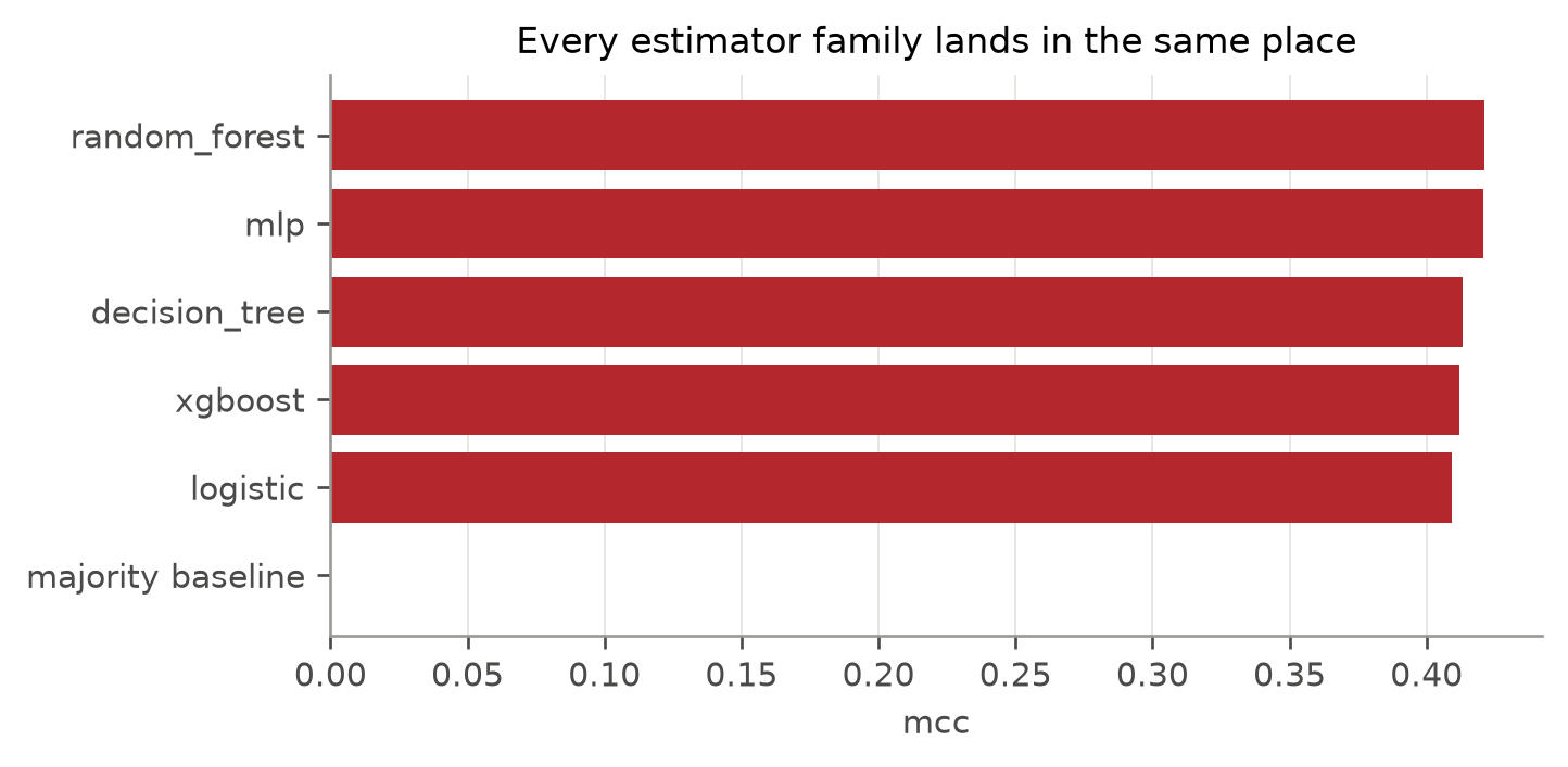
Answering it calls for trying differently rather than trying harder. Figure 3.2 fits several estimator families under identical preprocessing, identical folds and identical scoring. They have very different assumptions about what a decision boundary should look like: one is linear, one is a single tree, two are ensembles of trees, one is a small neural network.
| Estimator | Matthews correlation | Balanced accuracy | Macro F1 | Accuracy | Recall, serious or fatal |
|---|---|---|---|---|---|
| random_forest | 0.4212 | 0.4324 | 0.4491 | 0.8214 | 0.0017 |
| mlp | 0.4207 | 0.4346 | 0.4513 | 0.8210 | 0.0017 |
| decision_tree | 0.4133 | 0.4341 | 0.4528 | 0.8192 | 0.0102 |
| xgboost | 0.4121 | 0.4409 | 0.4621 | 0.8180 | 0.0204 |
| logistic | 0.4093 | 0.4299 | 0.4452 | 0.8183 | 0.0000 |
| majority baseline | 0.0000 | 0.3333 | 0.2897 | 0.7685 | 0.0000 |
If capacity were the binding constraint, adding capacity would help. It does not. The five families are separated by 0.0119 of Matthews correlation, which is less than the difference between any of them and a coin flip about which to use.
Nor does any of them win outright. On these figures random_forest leads on Matthews correlation while xgboost leads on recall for serious collisions and sits near the bottom on accuracy. The metrics disagree with each other more than the models do, which is the same point Appendix B makes about scoring: a single number is a choice about what to care about, not a fact about the model.
3.7.1 A correlation of 0.4 that means less than it looks
The Matthews correlation in that table is not small. Around 0.4 would ordinarily describe a model that was working, and the figure is no artifact: the baseline scores exactly zero by construction, so this is genuine agreement beyond what the base rates alone produce.
Read along the same row to the last column. Recall on serious and fatal collisions is at most 2.04%, and for two of the five families it is indistinguishable from zero.
Both figures are correct, and together they say what the model has actually learned. It separates collisions that hurt somebody from collisions that did not, with some success. It does almost nothing to separate the serious injuries from the minor ones. The three-level problem is being solved as a two-level one, and the level being skipped is the level that matters.
This is what one would expect from Chapter 2. After the pedestrian victim indicator was removed, the variables carrying most of the signal are the ones describing who was involved: the type of collision, and whether a cyclist or motorcyclist was among the parties. Those predict injury, because a person struck outside a vehicle usually is injured. They say very little about how badly, and nothing in the extract does.
Chapter 4 takes up which variables are doing this work, and whether any of them are variables anyone could change.
3.8 It is not the amount of data
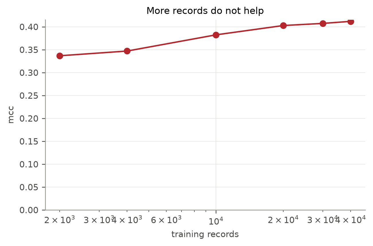
The other obvious objection is that more records would help. Figure 3.3 refits on growing fractions of the training data.
| Fraction used | Records | Matthews correlation | Balanced accuracy | Recall, serious or fatal |
|---|---|---|---|---|
| 0.05 | 2,000 | 0.3367 | 0.4316 | 0.0136 |
| 0.10 | 4,000 | 0.3470 | 0.4283 | 0.0085 |
| 0.25 | 10,000 | 0.3824 | 0.4341 | 0.0153 |
| 0.50 | 20,000 | 0.4027 | 0.4379 | 0.0153 |
| 0.75 | 30,000 | 0.4074 | 0.4372 | 0.0119 |
| 1.00 | 40,000 | 0.4118 | 0.4399 | 0.0170 |
The curve is not flat, and calling it flat would overstate the case. The Matthews correlation does rise as records are added, by +0.0103 over the first step of the table and by +0.0045 over the last. At the right-hand edge it is still rising.
What it is doing is flattening. Each addition buys less than the one before, which is the shape of a curve approaching an asymptote rather than one with room left to climb. Extrapolating it would be guesswork, so the reading here stays narrow: another decade of reports recorded the same way would move this number, and the four other arguments in this chapter are why it would not move far enough to matter.
3.9 Better than chance, and by how much
The phrase “better than chance” is a claim about a distribution, and it can be checked directly by destroying the relationship and measuring what survives.
Shuffling the outcomes leaves every marginal untouched. The same class imbalance, the same variables, the same number of records, the same cells. What it removes is any connection between a collision’s recorded circumstances and what happened to it. Whatever a procedure scores on shuffled outcomes is what it scores on nothing at all (Ojala & Garriga, 2010).
| Quantity | Observed | Shuffled outcomes | p |
|---|---|---|---|
| Accuracy bound, every cell counted | 0.9205 | 0.8980 | 0.024 |
| Cell-majority rule, scored on held-out records | 0.7778 | 0.7175 | 0.024 |
The first row is the promised demonstration. The bound computed over every cell barely changes when the outcomes are randomised, because it was never measuring predictability. It was measuring how many distinct combinations of variables exist, and shuffling the outcomes does not change that.
The second row is the real test, and licenses every statement about chance in this book.
3.10 What this amounts to
Four arguments, none of which depends on any of the others.
Cells of identically recorded collisions have mixed outcomes, so no method can separate them. Counting that across the data gives an upper bound on accuracy. Fano’s inequality gives a floor under the error rate from the information the variables carry. Five estimator families and a learning curve say the limit belongs to the data rather than to the model or the sample size.
They agree. What remains is to ask which variables are carrying what little there is, and whether any of them are variables anyone could act on.