# Worked examples {#sec-worked}
Three larger runs, putting the whole pipeline together at $e^{20}$ and $e^{21}$: many interval lengths at once, the alternative prediction $F^*$ on stage, and a nested animation. The heavy computations were run once and saved; the cells that took minutes to hours are displayed but not executed, and everything downstream retrieves from the database. The folded cell below defines the `pick` helper of @sec-retrieve.
{{< include _pick.qmd >}}
```{python}
import matplotlib.pyplot as plt

import primes_in_intervals as pii
from primes_in_intervals import (
    analyze,
    compare,
    intervals,
    nest,
    plot_distribution_frame,
    retrieve,
    save,
)
```
## Example 4 {#sec-eg4worked}
```{python}
# In this example, we'll try our alternative estimate F*(H,m,lambda*), lambda* = H/log N.
N = int(np.exp(20))
HH = [20,30,40,50,60,70,80,90,100,200]
step = 10**3
A = N - 10**5
B = N + 10**5
C = list(range(A,B+1,step))
```
Ten interval lengths over one pass each of half a billion integers: the computation below took a little under an hour, so it is shown, not run.
```{python}
#| eval: false
exp20 = { H : {} for H in HH}
start = timer()
for H in HH:
    exp20[H] = intervals(C,H,interval_type='overlap')
end = timer()
end - start
```
```
3146.539329699939
```
```{python}
#| eval: false
for H in HH:
    save(exp20[H])
```
Retrieval brings all ten datasets back. Other datasets share some of these interval lengths, so, as always, we select by lower bound with `pick` rather than by position; the printed summaries list everything each length matched.
```{python}
getexp20 = {}
for H in HH:
    getexp20[H] = pick(retrieve(H), A)
```
```{python}
for H in HH:
    analyze(getexp20[H])
```
```{python}
for H in HH:
    compare(getexp20[H])
```
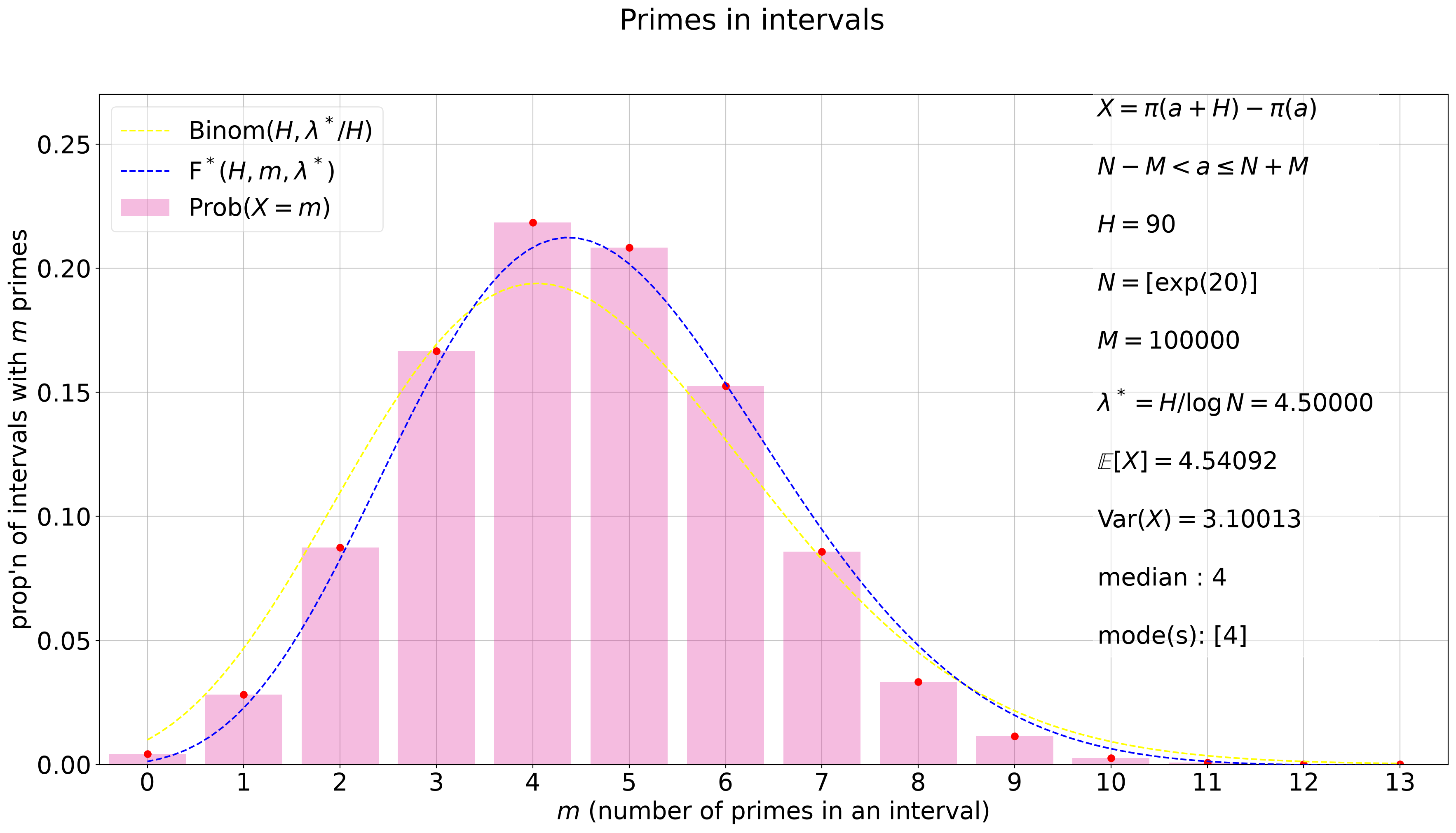
Now the plot, for $H = 90$: this is the figure where the alternative pair takes the stage, $\mathrm{Binom}(H, \lambda^*/H)$ and $F^*(H,m,\lambda^*)$ with $\lambda^* = H/\log N$, in place of the usual pair. The final frame's text box states the range in its centered form, so we pass the overlay as a literal string.
```{python}
H = 90 # 20,30,40,50,70,80,200
X = getexp20[H]

A = X['header']['lower_bound']
H = X['header']['interval_length']
C = list(X['distribution'].keys())
B = C[-1]

N = (A + B)/2
p_alt = 1/np.log(N)
mu = X['statistics'][B]['mean']
sigma = X['statistics'][B]['var']
med = X['statistics'][B]['med']
if med == int(med):
    med = int(med)
modes = X['statistics'][B]['mode']

overlay_text = (fr'$X = \pi(a + H) - \pi(a)$' + '\n\n'
                + fr'$N - M < a \leq N + M$' + '\n\n'
                + fr'$H = {H}$' + '\n\n'
                + fr'$N = [\exp(20)]$' + '\n\n'
                + fr'$M = {int(B - N)}$' + '\n\n'
                + fr'$\lambda^* = H/\log N = {H*p_alt:.5f}$' + '\n\n'
                + r'$\mathbb{E}[X] = $' + f'{mu:.5f}' + '\n\n'
                + r'$\mathrm{Var}(X) = $' + f'{sigma:.5f}' + '\n\n'
                + fr'median : ${med}$' + '\n\n'
                + fr'mode(s): ${modes}$')

plt.rcParams.update({'font.size': 22})
fig, ax = plt.subplots(figsize=(22, 11))
fig.suptitle('Primes in intervals')
plot_distribution_frame(ax, X, B,
                        show_binom=False, show_binom_alt=True,
                        show_frei=False, show_frei_alt=True,
                        overlay=overlay_text, overlay_position=(0.74, 0.18))
plt.rcParams['savefig.facecolor'] = 'white'
plt.show()
```
## Example 5 {#sec-eg5worked}
The same window about $e^{20}$, now at the single length $H = 76$. The computation ran once (several minutes) and was saved:
```{python}
#| eval: false
N = int(np.exp(20))
M = 10**5
H = 76
A = N - M
B = N + M
step = 10**3
C = list(range(A, B + 1, step))
N_exp20_H_76 = intervals(C, H)
```
```{python}
N_exp20_H_76 = pick(retrieve(76), 485065195)
```
```{python}
analyze(N_exp20_H_76)['header']
```
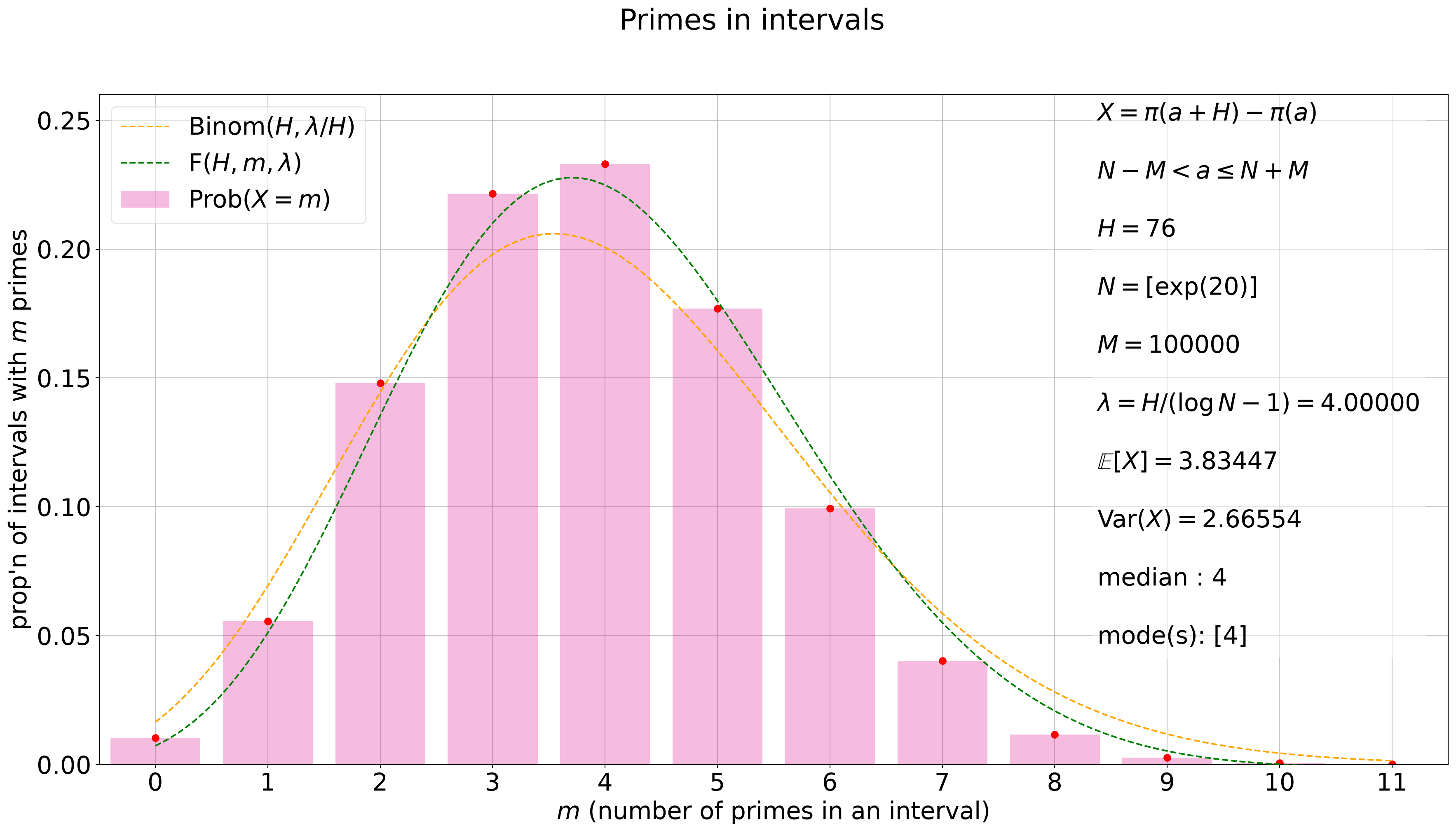
The plot is the standard pair, $\mathrm{Binom}(H, \lambda/H)$ against $F(H,m,\lambda)$, with the centered overlay on the final frame.
```{python}
X = N_exp20_H_76

A = X['header']['lower_bound']
H = X['header']['interval_length']
C = list(X['distribution'].keys())
B = C[-1]

N = (A + B)/2
p = 1/(np.log(N) - 1)
mu = X['statistics'][B]['mean']
sigma = X['statistics'][B]['var']
med = X['statistics'][B]['med']
if med == int(med):
    med = int(med)
modes = X['statistics'][B]['mode']

overlay_text = (fr'$X = \pi(a + H) - \pi(a)$' + '\n\n'
                + fr'$N - M < a \leq N + M$' + '\n\n'
                + fr'$H = {H}$' + '\n\n'
                + fr'$N = [\exp(20)]$' + '\n\n'
                + fr'$M = {int(B - N)}$' + '\n\n'
                + fr'$\lambda = H/(\log N - 1) = {H*p:.5f}$' + '\n\n'
                + r'$\mathbb{E}[X] = $' + f'{mu:.5f}' + '\n\n'
                + r'$\mathrm{Var}(X) = $' + f'{sigma:.5f}' + '\n\n'
                + fr'median : ${med}$' + '\n\n'
                + fr'mode(s): ${modes}$')

fig, ax = plt.subplots(figsize=(22, 11))
fig.suptitle('Primes in intervals')
plot_distribution_frame(ax, X, B, overlay=overlay_text, overlay_position=(0.74, 0.18))
plt.show()
```
The full animation is saved with `save_gif` or `save_mp4` (or `pii animate`); the frames step through the two hundred checkpoints of the window.
## Example 6 (nested intervals) {#sec-eg6worked}
The largest run: nested intervals about $e^{21}$, thirteen interval lengths from $20$ to $140$. The checkpoints are placed symmetrically about $N$, a thousand apart, with $N$ itself excluded, so that nesting pairs them off exactly.
```{python}
N = int(np.exp(21))
K = 199
k = (K - 1)//2 # = 99
Delta = 10**3
D = []
for j in range(k + 1):
    D.extend([N - (j + 1)*Delta, N + (j + 1)*Delta])
C = sorted(D)
HH = list(range(20,141,10))
```
```{python}
#| eval: false
EXP21 = {H : {} for H in HH}
for H in HH:
    EXP21[H] = intervals(C, H)
# Takes a few hours...
```
```{python}
#| eval: false
for H in HH:
    save(EXP21[H])
```
```{python}
EXP21 = {}
for H in HH:
    EXP21[H] = pick(retrieve(H), C[0])
```
```{python}
NEXP21 = {}
for H in HH:
    NEXP21[H] = nest(EXP21[H])
for H in HH:
    analyze(NEXP21[H])
```
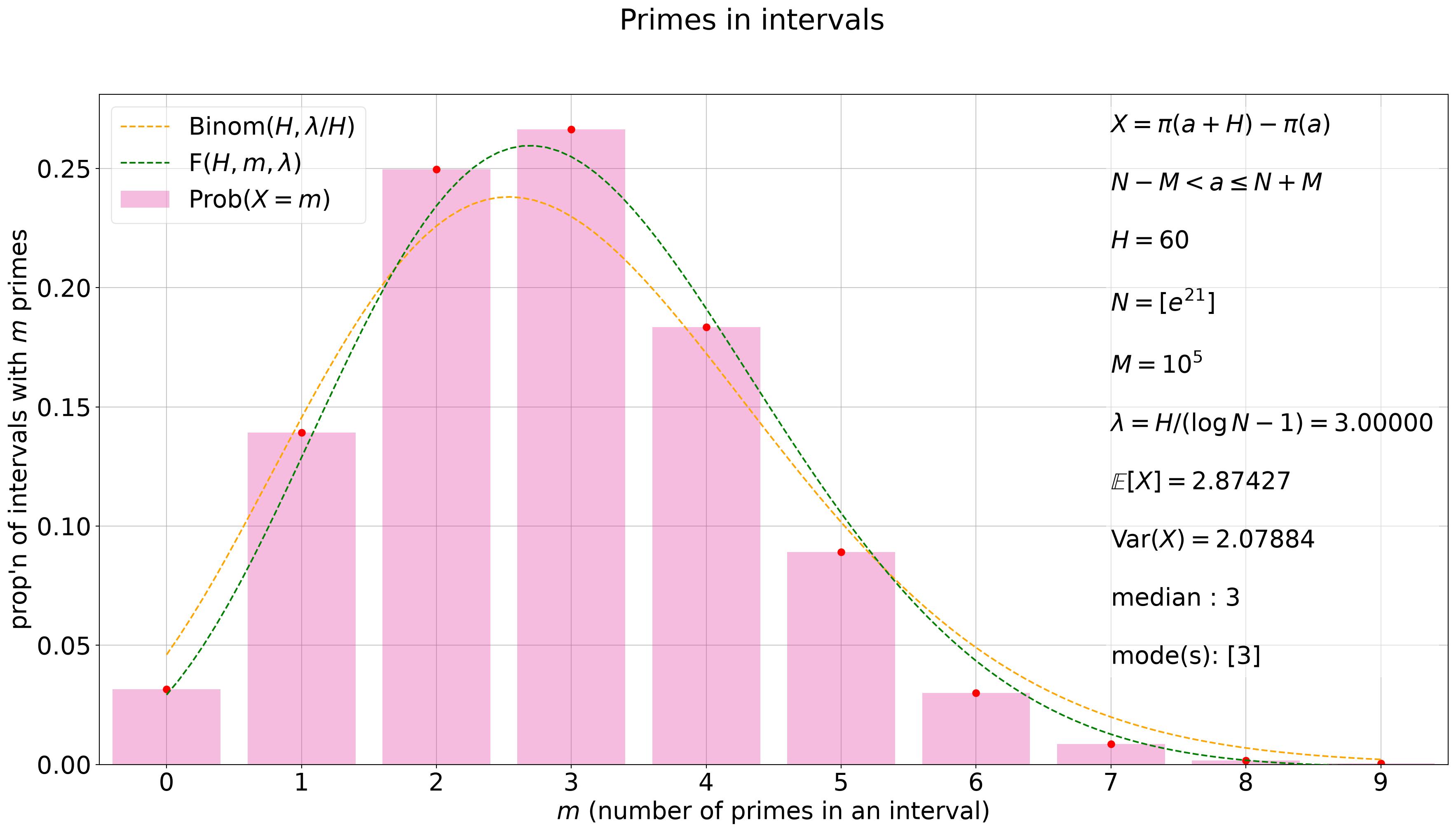
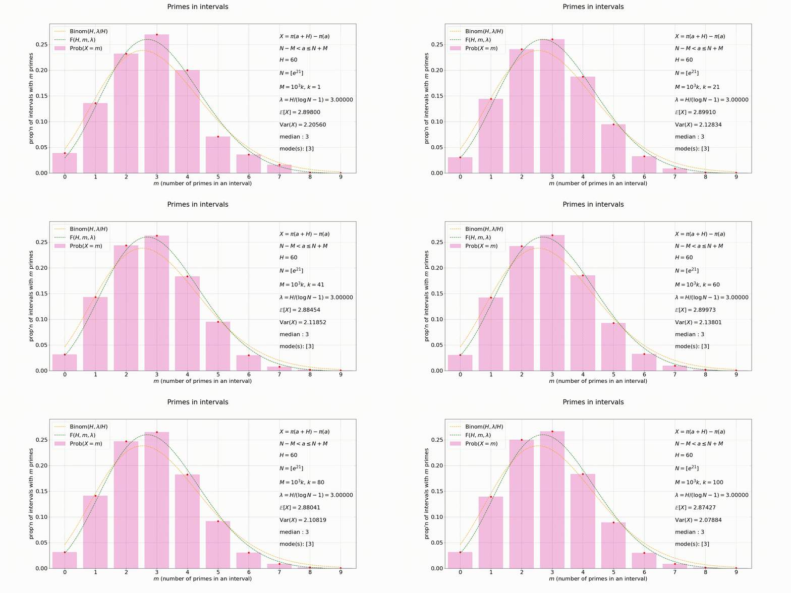
The plot, for $H = 60$, is the nested version: each frame is one of the hundred nested intervals, the innermost first, the sample growing outward from the midpoint, with the vertical axis rounded at the third decimal for these smaller proportions.
```{python}
# HH = [20, 30, 40, 50, 60, 70, 80, 90, 100, 110, 120, 130, 140]
X = NEXP21[HH[4]]

H = X['header']['interval_length']
C = list(X['distribution'].keys())
c = C[-1]

A = c[0]
B = c[1]
N = (A + B)//2
p = 1/(np.log(N) - 1)
mu = X['statistics'][c]['mean']
sigma = X['statistics'][c]['var']
med = X['statistics'][c]['med']
if med == int(med):
    med = int(med)
modes = X['statistics'][c]['mode']

overlay_text = (fr'$X = \pi(a + H) - \pi(a)$' + '\n\n'
                + fr'$N - M < a \leq N + M$' + '\n\n'
                + fr'$H = {H}$' + '\n\n'
                + r'$N = [e^{21}]$' + '\n\n'
                + fr'$M = 10^5$' + '\n\n'
                + fr'$\lambda = H/(\log N - 1) = {H*p:.5f}$' + '\n\n'
                + r'$\mathbb{E}[X] = $' + f'{mu:.5f}' + '\n\n'
                + r'$\mathrm{Var}(X) = $' + f'{sigma:.5f}' + '\n\n'
                + fr'median : ${med}$' + '\n\n'
                + fr'mode(s): ${modes}$')

plt.rcParams.update({'font.size': 22})
fig, ax = plt.subplots(figsize=(22, 11))
fig.suptitle('Primes in intervals')
plot_distribution_frame(ax, X, c, ylim_decimals=3,
                        overlay=overlay_text, overlay_position=(0.75, 0.15))
plt.rcParams['savefig.facecolor'] = 'white'
plt.show()
```
The animation, innermost interval outward:
{fig-alt="Animation of the distribution of primes in intervals of length 60 about e^21, the nested sample growing outward from the midpoint, with the Binomial and F prediction curves overlaid."}
## Supplementary examples {#sec-supplementary}
Four further examples, at sizes where everything runs in seconds, so every cell below computes live: the Nachlass tables in full, the nested pipeline at $e^{17}$ for overlapping and for prime-starting intervals, and a closing remark on the choice of $\lambda$. (These complement @sec-eg3display's one-line Goldschmidt table.)
### Example 1 {#sec-eg1supp}
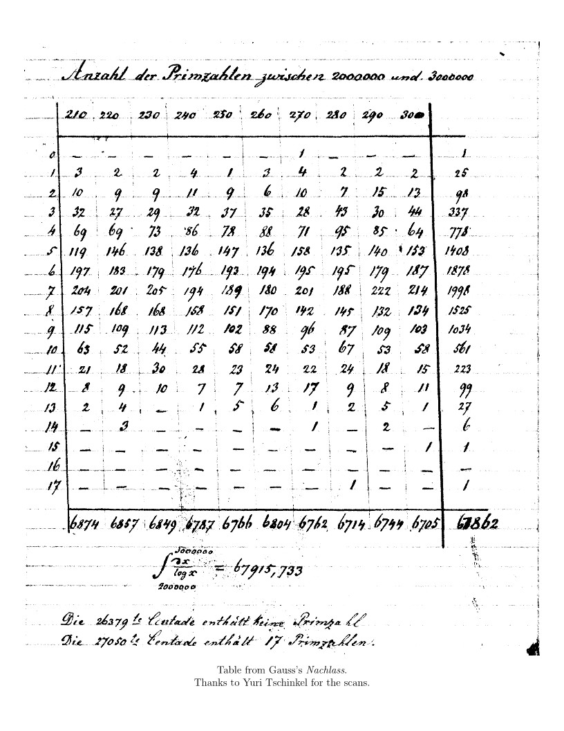
Tables from Gauss's _Nachlass_. Create data for primes in disjoint intervals of length $100$ (starting at multiples of $100$), up to $10^7$. Checkpoints every $10^5$.
By the bye, an interval of the form $[100k, 100k + 100)$ is referred to as a "Centade" in Gauss's _Nachlass_. Analogous to the term Decade (a 10-year period from years '0 to '9), a Centade is a 100-year period from '00 to '99.
```{python}
C = list(range(0,10*10**6 + 1, 10**5))
H = 100
nachlass = pii.intervals(C,H,'disjoint')
```
Gauss and Goldschmidt summarize their data in tables of primes up to $1$ million, between $1$ and $2$ million, and so on. Let's emulate that.
```{python}
NACHLASS = { }
for i in range(1,11):
    NACHLASS[i] = pii.extract(nachlass, [(i - 1)*10**6, i*10**6] , option='narrow')
    pii.partition(NACHLASS[i])
```
Let's display one of these tables: the one for primes between $2$ and $3$ million.
```{python}
NACHLASS3df = pii.display(NACHLASS[3], count='partition', orient='columns')
NACHLASS3df
```
Here's the original: Gauss/Goldschmidt were only short by $21$ primes in the end!
{fig-alt="Facsimile of the Nachlass table tallying primes per Centade between two and three million."}
### Example 2 {#sec-eg2supp}
Let's look at a series of nested intervals centred around $N = [e^{17}] = 24,154,952$. We take the density of primes close to $N$ as $1/(\log N - 1)$, which is $1/15.999999968802452\ldots$, virtually $1/16$. We'll get data for intervals of length $64, 68, 72, 76, 80$.
```{python}
N = int(np.exp(17))
HH = [64, 68, 72, 76, 80]
C = list(range(N - 10**4,N + 10**4 + 1, 10**2))
EXP17 = {}
for H in HH:
    EXP17[H] = pii.intervals(C, H, 'overlap')
```
Right now we have data for the intervals $(N - 10^4, N - 10^4 + 100k]$, $k = 1,\ldots,100$. Let's reconfigure the data to consider nested intervals $(N - 100k, N + 100k]$, $k = 1,\ldots,100$, all centred around $N$. We'll analyze the data (get the distributions and statistics) while we're at it.
```{python}
EXP17NEST = {}
for H in HH:
    EXP17NEST[H] = pii.nest(EXP17[H])
    pii.analyze(EXP17NEST[H])
```
Let's display what we have for $H = 76$ for instance.
```{python}
EXP17_76_NESTtable = pii.display(EXP17NEST[76])
EXP17_76_NESTtable.tail(5)
```
Let's compare the data (for $H = 76$) to three predictions: the Binomial, our prediction, and the alternate version of our prediction (with the density of primes around $N$ taken to be $1/\log N$). Specifically, with $\lambda = H/(\log N - 1)$ (and assuming $\lambda \asymp 1$), the naive prediction based purely on Cramér's model is the Binomial distribution $\mathrm{Binom}(H,\lambda/H)$, whose probability mass function is given by
$$f(m; H, \lambda/H) = \binom{H}{m}\left(\frac{\lambda}{H}\right)^m\left(1 - \frac{\lambda}{H}\right)^{H - m} = \frac{e^{-\lambda}\lambda^m}{m!}\bigg[1 + \frac{Q_1(\lambda,m)}{H} + \frac{Q_2(\lambda,m)}{H^2} + \cdots\bigg],$$
where each $Q_j(\lambda,m)$ is a polynomial in $\lambda$ and $m$, and in particular,
$$Q_1(\lambda,m) = \frac{m - (m - \lambda)^2}{2}.$$
Our prediction is
$$F(H,m,\lambda) = \frac{e^{-\lambda}\lambda^m}{m!}\left[1 + \frac{Q_1(\lambda,m)}{H}\left(\log H + (\log 2\pi + \gamma - 1)\right) \right].$$
Our alternative prediction is, with $\lambda^* = H/\log N$,
$$F^*(H,m,\lambda^*) = \frac{e^{-\lambda^*}(\lambda^*)^m}{m!}\left[1 + \frac{\lambda^*}{H}(m - \lambda^*) + \frac{\log H + (\log 2\pi + \gamma - 1)}{H}Q_1(m,\lambda^*) \right].$$
The table below shows tuples $(a,b,c,d)$, where $a$ is the actual number, $b$ is the Binomial-based prediction, $c$ is our prediction and $d$ is our alternative prediction. It would be nice to be able to conjecture something about a tertiary term!
We'll just show the last five rows of the table as it's a bit long and hard to read.
```{python}
pii.compare(EXP17NEST[76])
EXP17_76_NESTcompare = pii.display(EXP17NEST[76], comparisons='absolute').tail(5)
EXP17_76_NESTcompare
```
We can perhaps work on the formatting of such tables.
Now, we want to know which prediction is the "best", and this is hard to see by glancing at the above table. By "best" we mean gives the smallest sum-of-squared-error over $m$ (number of primes in an interval). We're mainly interested in comparing $F$ and $F^*$. Comparing $F^*$ to the Binomial is not really apples-to-apples because the Binomial we are using takes the probability of finding a prime around $N$ as being $\lambda/H = 1/(\log N - 1)$, rather than $\lambda^*/H = 1/\log N$, as in $F^*$.
We'll use our ```winners``` function to determine the best predictions for each interval. For each prediction, this function also gives us the $m$ for which that prediction gives a smaller error than the others.
```{python}
pii.winners(EXP17NEST[76])
EXP17_76_NESTwinners = pii.display(EXP17NEST[76], winners='show')
EXP17_76_NESTwinners.tail(10)
```
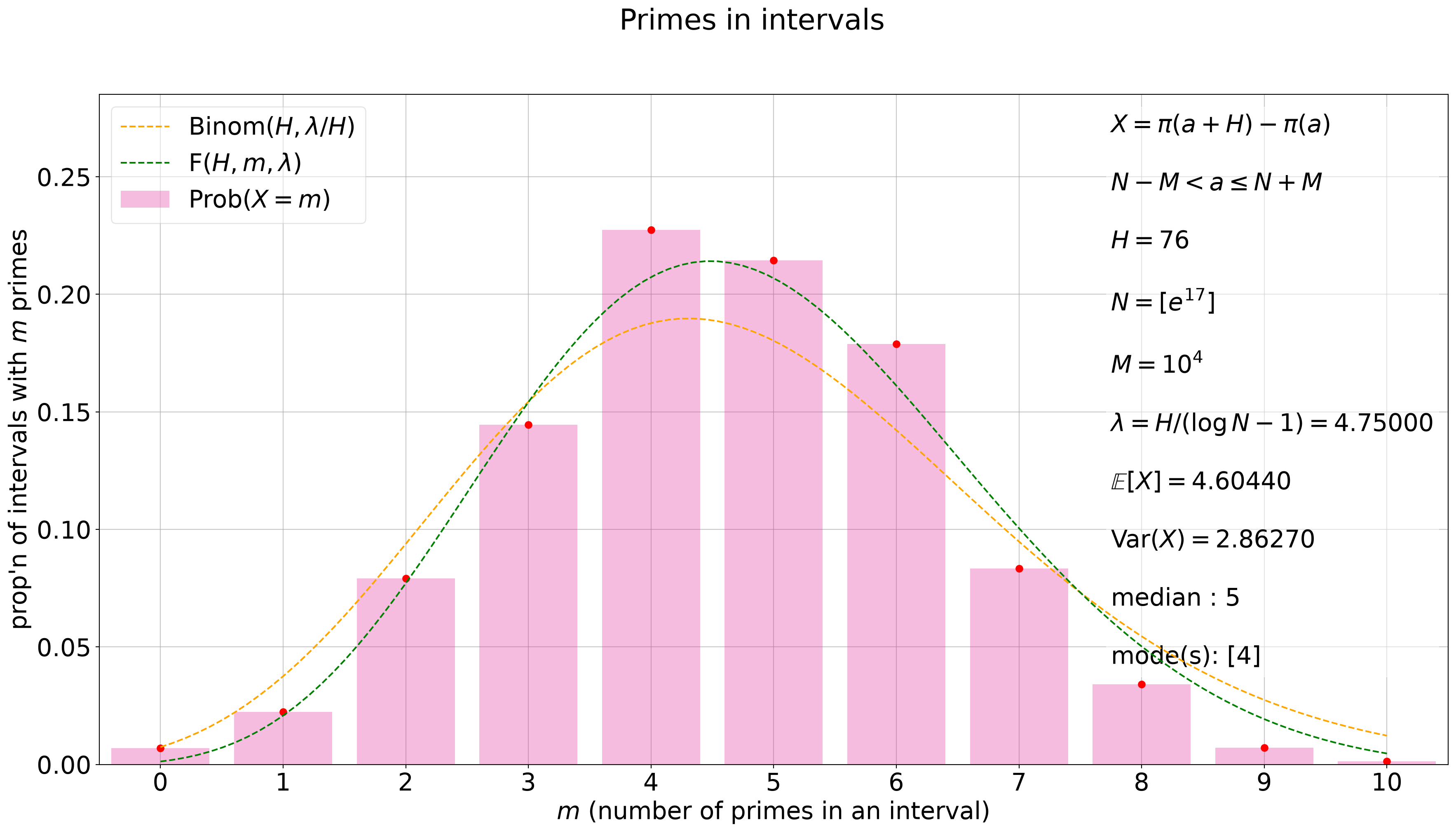
Finally, let's make an animated plot, with one frame for each of the intervals considered. Here is its final frame, drawn live:
```{python}
# HH = [64, 68, 72, 76, 80]
X = EXP17NEST[HH[3]]

H = X['header']['interval_length']
C = list(X['distribution'].keys())
c = C[-1]

A = c[0]
B = c[1]
N = (A + B)//2
p = 1/(np.log(N) - 1)
mu = X['statistics'][c]['mean']
sigma = X['statistics'][c]['var']
med = X['statistics'][c]['med']
if med == int(med):
    med = int(med)
modes = X['statistics'][c]['mode']

overlay_text = (fr'$X = \pi(a + H) - \pi(a)$' + '\n\n'
                + fr'$N - M < a \leq N + M$' + '\n\n'
                + fr'$H = {H}$' + '\n\n'
                + r'$N = [e^{17}]$' + '\n\n'
                + fr'$M = 10^4$' + '\n\n'
                + fr'$\lambda = H/(\log N - 1) = {H*p:.5f}$' + '\n\n'
                + r'$\mathbb{E}[X] = $' + f'{mu:.5f}' + '\n\n'
                + r'$\mathrm{Var}(X) = $' + f'{sigma:.5f}' + '\n\n'
                + fr'median : ${med}$' + '\n\n'
                + fr'mode(s): ${modes}$')

plt.rcParams.update({'font.size': 22})
fig, ax = plt.subplots(figsize=(22, 11))
fig.suptitle('Primes in intervals')
plot_distribution_frame(ax, X, c, ylim_decimals=3,
                        overlay=overlay_text, overlay_position=(0.75, 0.15))
plt.rcParams['savefig.facecolor'] = 'white'
plt.show()
```
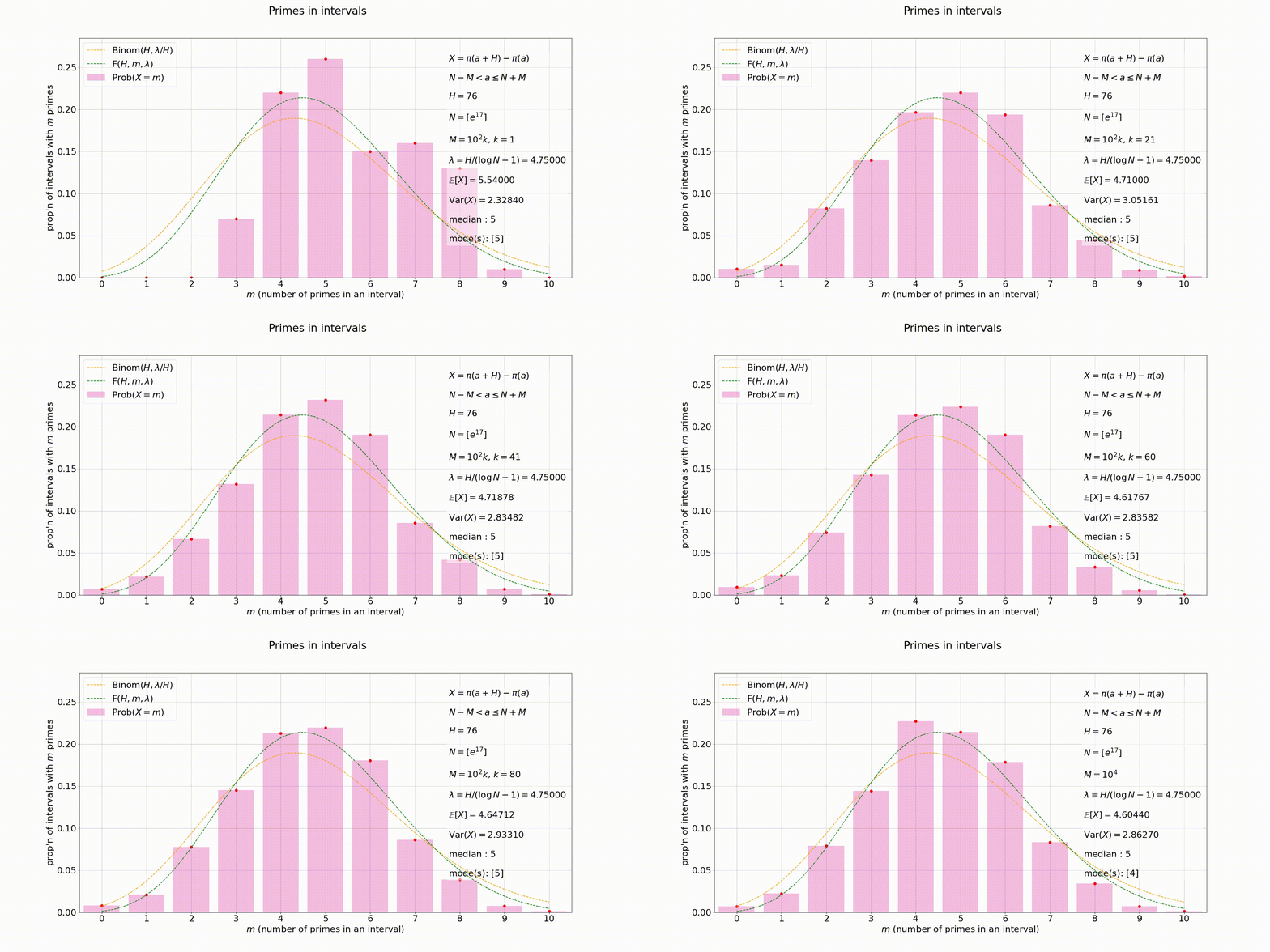
And the animation itself:
{fig-alt="Animation of the distribution of primes in intervals of length 76 about e^17, the nested sample growing outward, with the Binomial and F curves overlaid."}
### Example 3 {#sec-eg3supp}
Let's go through the steps of [Example 2](#sec-eg2supp), but instead of counting all intervals of the form $(a, a + H]$ as $a$ runs over all integers in the range $(N - M, N + M]$, let's consider only intervals of the form $(p, p + H]$ as $p$ runs over only the _primes_ in the range $(N - M, N + M]$. We have not yet worked through the details of the second-order term in our prediction in this case, but up to first order approximation we should still have $e^{-\lambda}\lambda^m/m!$...
First we generate the data using the ```'prime_start'``` option in our ```intervals``` function.
```{python}
N = int(np.exp(17))
HH = [64, 68, 72, 76, 80]
C = list(range(N - 10**4,N + 10**4 + 1, 10**2))
PSEXP17 = {}
for H in HH:
    PSEXP17[H] = pii.intervals(C, H, 'prime_start')
```
Let's centre the intervals around $N$ with the ```nest``` function.
```{python}
PSEXP17NEST = {}
for H in HH:
    PSEXP17NEST[H] = pii.nest(PSEXP17[H])
    pii.analyze(PSEXP17NEST[H])
```
Let's have a look at the data in a table.
```{python}
PSEXP17_76_NESTtable = pii.display(PSEXP17NEST[76])
PSEXP17_76_NESTtable.tail(5)
```
Although our predictions have only been worked out for the case of overlapping intervals, and the secondary term in the case of disjoint/left-endpoint-prime intervals might well be a bit different, we can nevertheless compare the data to these "predictions"...
```{python}
pii.compare(PSEXP17NEST[76])
PSEXP17_76_NESTcompare = pii.display(PSEXP17NEST[76], comparisons='absolute').tail(5)
PSEXP17_76_NESTcompare
```
...and see which not-really-a-prediction fares best...
```{python}
pii.winners(PSEXP17NEST[76])
PSEXP17_76_NESTwinners = pii.display(PSEXP17NEST[76], winners='show')
PSEXP17_76_NESTwinners.tail(10)
```
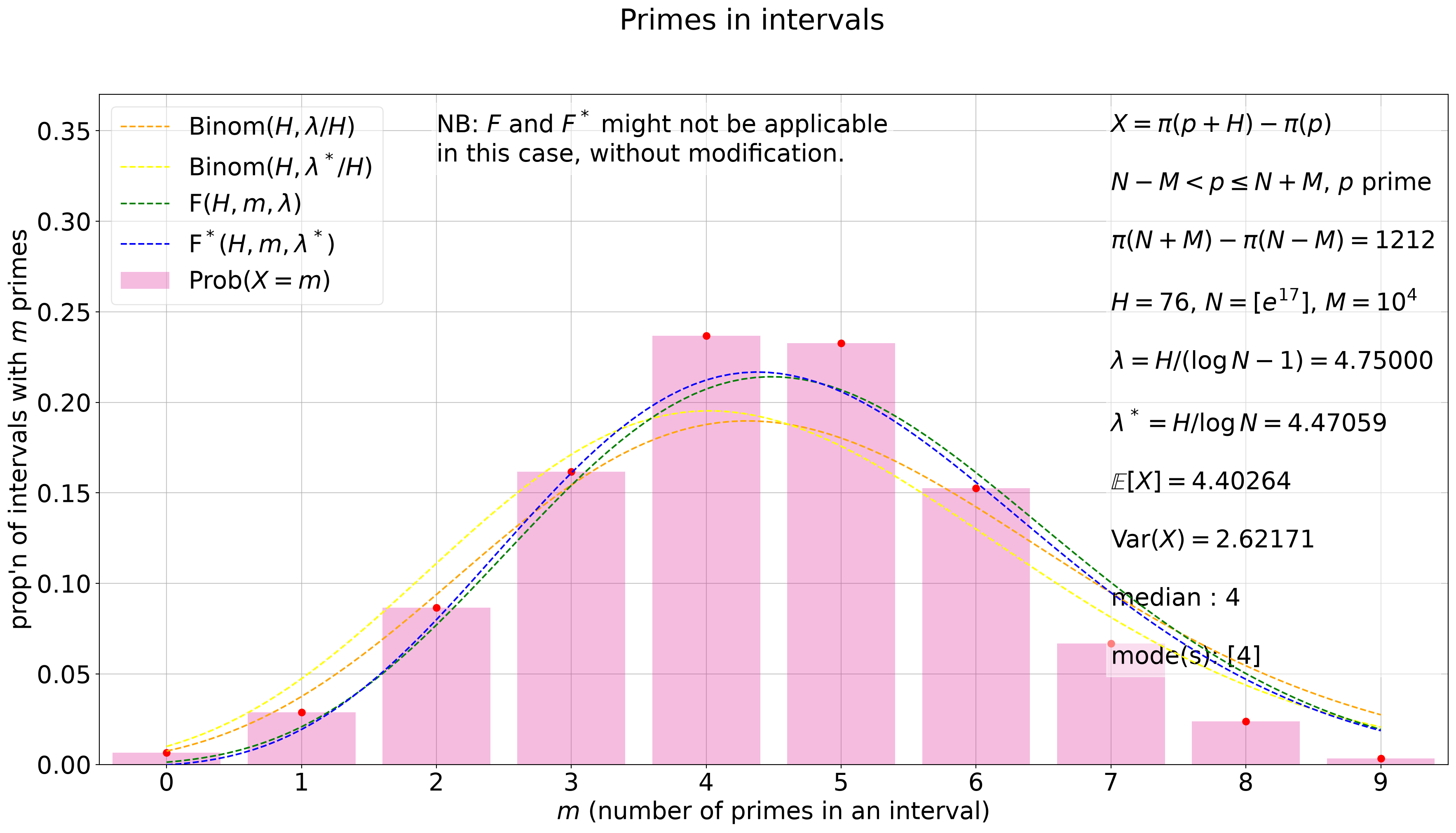
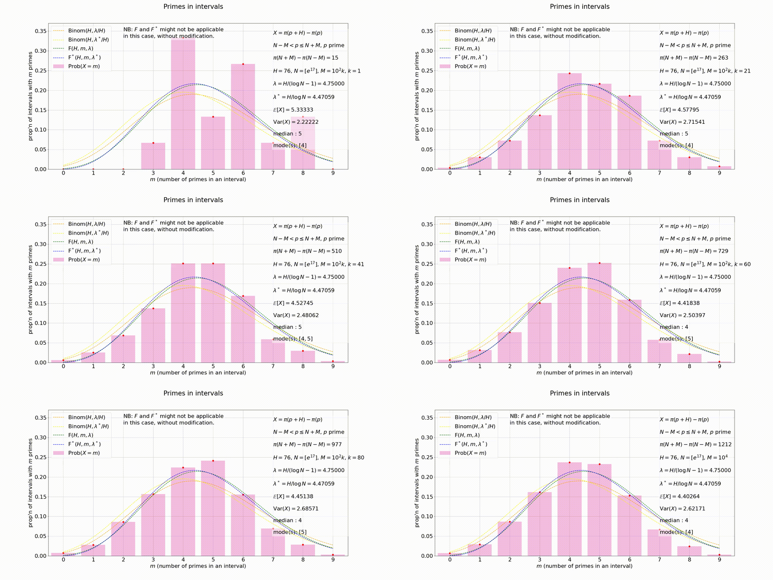
And now we can grok everything with an animation... Actually, these not-necessarily-predictions look half-decent, given that there are only about $1000$ intervals being used for the data. Here, all four curves are drawn, the standard pair and the alternative pair, with a caveat boxed at the top; the final frame:
```{python}
# HH = [64, 68, 72, 76, 80]
X = PSEXP17NEST[HH[3]]

H = X['header']['interval_length']
C = list(X['distribution'].keys())
c = C[-1]

A = c[0]
B = c[1]
N = (A + B)//2
PI = sum(X['nested_interval_data'][c].values())
p = 1/(np.log(N) - 1)
p_alt = 1/(np.log(N))
mu = X['statistics'][c]['mean']
sigma = X['statistics'][c]['var']
med = X['statistics'][c]['med']
if med == int(med):
    med = int(med)
modes = X['statistics'][c]['mode']

overlay_text = (fr'$X = \pi(p + H) - \pi(p)$' + '\n\n'
                + fr'$N - M < p \leq N + M$, $p$ prime' + '\n\n'
                + fr'$\pi(N + M) - \pi(N - M) = {PI}$' + '\n\n'
                + fr'$H = {H}$, '
                + r'$N = [e^{17}]$, '
                + fr'$M = 10^4$' + '\n\n'
                + fr'$\lambda = H/(\log N - 1) = {H*p:.5f}$' + '\n\n'
                + fr'$\lambda^* = H/\log N = {H*p_alt:.5f}$' + '\n\n'
                + r'$\mathbb{E}[X] = $' + f'{mu:.5f}' + '\n\n'
                + r'$\mathrm{Var}(X) = $' + f'{sigma:.5f}' + '\n\n'
                + fr'median : ${med}$' + '\n\n'
                + fr'mode(s): ${modes}$')

fig, ax = plt.subplots(figsize=(22, 11))
fig.suptitle('Primes in intervals')
plot_distribution_frame(ax, X, c,
                        show_binom_alt=True, show_frei=True, show_frei_alt=True,
                        note='NB: $F$ and $F^*$ might not be applicable' + '\n' + 'in this case, without modification.',
                        overlay=overlay_text, overlay_position=(0.75, 0.15))
plt.show()
```
{fig-alt="Animation of the distribution of primes in intervals of length 76 whose left endpoints are prime, about e^17, with all four prediction curves overlaid and a caveat that F and F* may not apply."}
### Example 4 {#sec-eg4supp}
We use $\lambda = H/(\log N - 1)$ in our prediction $F(H,m,\lambda)$ because the density of primes close to $N$ is approximately $1/(\log N - 1)$, by the prime number theorem. Actually, the prime number theorem says that the number of primes up to $N$ is well-approximated by
$$\int_2^N \frac{dt}{\log t} = \frac{N}{\log N} + \frac{N}{(\log N)^2} + \frac{2N}{(\log N)^3} + \cdots .$$
Thus, the average density of primes up to $N$ is approximated by
$$\frac{1}{N} \int_2^N \frac{dt}{\log t} = \frac{1}{\log N} + \frac{1}{(\log N)^2} + \frac{2}{(\log N)^3} + \cdots .$$
(Indeed, Gauss's observation from his numerical data was that the density of primes around $n$ is around $1/\log n$, so that the number of primes around $N$ may be estimated by integrating over this density.) Notice that
$$\frac{1}{\log N - 1} = \frac{1}{\log N} + \frac{1}{(\log N)^2} + \frac{1}{(\log N)^3} + \cdots, $$
and so $1/(\log N - 1)$ is a good proxy for what the prime number theorem gives us: more precisely,
$$\frac{1}{N} \int_2^N \frac{dt}{\log t} = \frac{1}{\log N - 1} + O\left(\frac{1}{(\log N)^3}\right).$$
In fact, the details leading to our prediction $F(H,m,\lambda)$ are unaffected if, instead of letting $\lambda = H/(\log N - 1)$, we let $\lambda = H/(\log N - 1 + \epsilon(N))$, where $\epsilon(N) \to 0$ rapidly enough. (This is also related to the reason why, if we let $\lambda^* = H/\log N$, which only approximates what we get from the logarithmic integral up to an error of $O(1/(\log N)^2)$, we get a different form for our prediction, which we are calling $F^*(H,m,\lambda^*)$.) That is, we can use better approximations than $1/(\log N - 1)$ to the density of primes close to $N$, but this does not affect the form of our prediction $F(H,m,\lambda)$, because $\epsilon(N)$ gets absorbed into our error terms. If we could work out or conjecture tertiary and higher order terms in our prediction $F(H,m,\lambda)$, this would become quite relevant and interesting.
Notwithstanding, we can still play around with $\lambda$ in our numerics. The prime number theorem suggests that if we are considering primes in intervals around $(N - M, N + M]$, we should take the density of primes (or "probability" of a random integer in the interval being prime) as
$$\frac{1}{2M} \int_{N - M}^{N + M} \frac{dt}{\log t}.$$
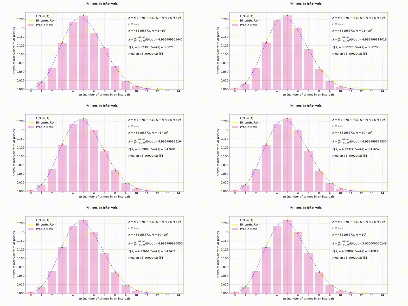
Again, letting this be $\lambda/H$ doesn't affect the form of our prediction $F(H,m,\lambda)$. Below is an animated plot, where we chose $N$ so that the above with $M = 10^6$ is very close to $1/20$.
{fig-alt="Animation of the distribution of primes in intervals of length 100, the density parameter chosen via the logarithmic integral to be very close to one twentieth."}
What we should really like to do is, instead of fixing $H$ and letting $\lambda = H/(\log N - 1)$ (or any of the alternatives above), and considering intervals close enough to $N$ that $\lambda$ remains more or less constant, is _fix_ $\lambda$, and let $H = \lambda \log n$ (say), where we are considering intervals of the form $(n, n + H]$. Then we'd have $\lambda/H = 1/\log n$, and this is what the prime number theorem (and Gauss) really say: the density of primes around an integer $n$ is $1/\log n$. Alas, for now, the argument leading to our prediction relies on the fact that $H$ is a fixed integer of size of order $\log N$.