2 Introduction
Excerpt from letter from Gauss to his student Johann Franz Encke, December 24, 1849 (see (Tschinkel 2006)).
In 1811, the appearance of Chernau’s cribrum gave me much pleasure and I have frequently (since I lack the patience for a continuous count) spent an idle quarter of an hour to count another chiliad here and there; although I eventually gave it up without quite getting through a million. Only some time later did I make use of the diligence of Goldschmidt to fill some of the remaining gaps in the first million and to continue the computation according to Burkhardt’s tables. Thus (for many years now) the first three million have been counted and checked against the integral. A small excerpt follows…
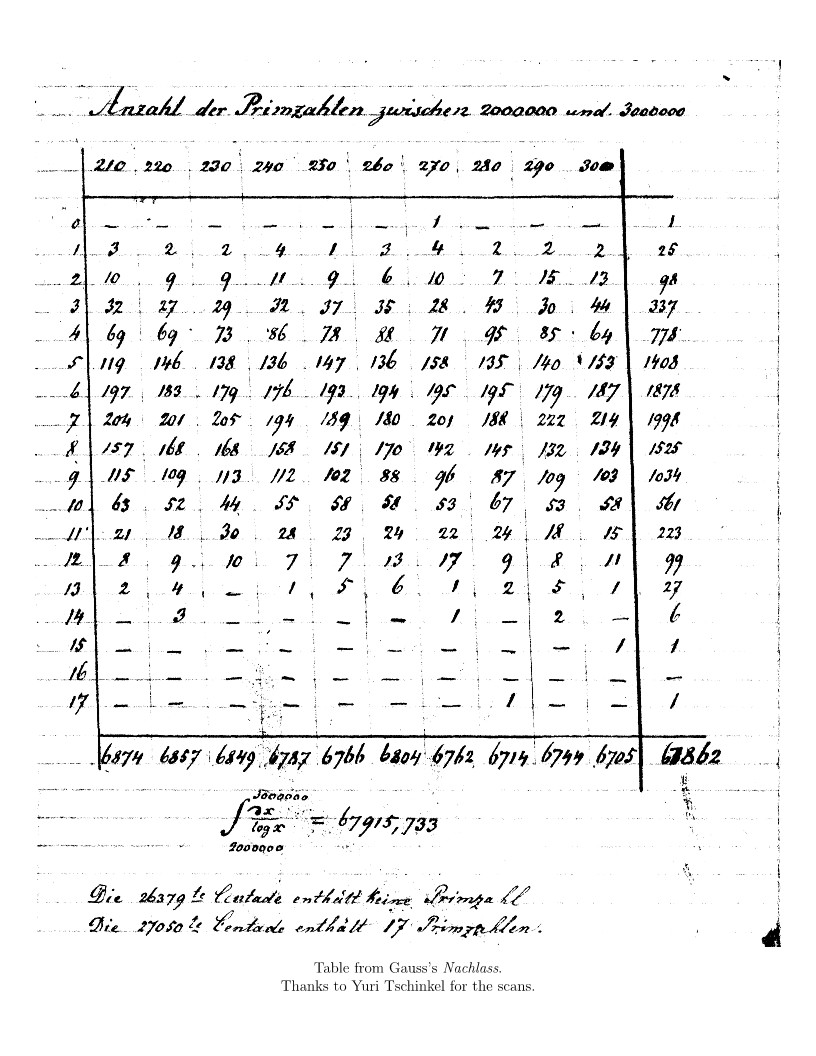
Gauss considered intervals \([0,100), [100,200), [200,300), \ldots\), which he called “centades” (a decade is a 10-year period from ’0 to ’9, a centade is a 100-year period from ’00 to ’99). He (and Goldschmidt) kept a tally of the number of centades that contain exactly \(m\) primes, for \(m = 0, 1, \ldots\). In Figure 2.1, we see the data for primes between \(2\) and \(3\) million. The row labels are \(m = 0,1,2,\ldots,17\). Then we have ten columns, the first for the range \(200 \times 10^5\) to \(210 \times 10^5\), then second for the range \(210 \times 10^5\) to \(220 \times 10^5\), and so on. In row \(m\), column \(n\), we have the number of centades between \((200 + 10(n - 1))\times 10^5\) and \((200 + 10n)\times 10^5\) that contain exactly \(m\) primes. The additional column on the right shows the row sums, giving the total number of centades between \(2\) and \(3\) million that contain a given number of primes. The weighted sum over this extra column, where the term corresponding to row \(m\) is weighted by \(m\), gives the total number of primes between \(2\) and \(3\) million.
What this allowed Gauss to notice is that the density of primes around \(n\) is approximately \(1/\log n\). For instance, we see that the average number of primes in a centade between \(2\) and \(3\) million is between \(6\) and \(7\), as is \(100/\log n\) for \(n\) between \(2\) and \(3\) million. Thus, Gauss conjectured that the number of primes up to \(N\) ought to be well approximated by integrating over this density:
\[\pi(N) = \#\{p \le N : p \textrm{ prime}\} \approx \int_2^N \frac{dt}{\log t}.\]
We can see that Gauss/Goldschmidt were comparing their data against this prediction. Gauss’s conjecture would become the prime number theorem in 1896, arguably the pinnacle of 19th century mathematics, when Hadamard and de la Vallée Poussin completed the program outlined by Riemann in his seminal 1859 manuscript. In fact, if the Riemann hypothesis is true, then
\[\pi(N) = \int_2^N \frac{dt}{\log t} + O\left(\sqrt{N}\log N\right).\]
Incidentally, here is the corrected table from Gauss’s Nachlass.
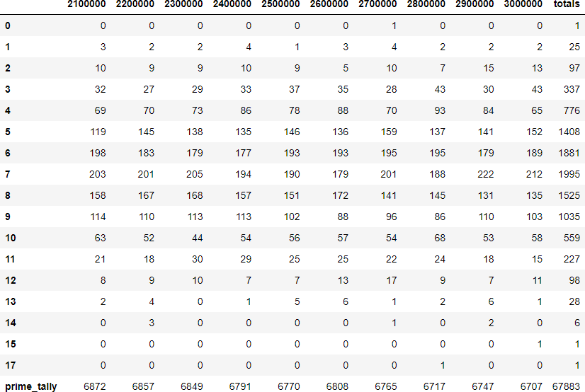
We can see that Gauss/Goldschmidt were only short by \(21\) primes in the end: not bad!
What we are interested in here is not just the average number of primes in a centade, but the distribution of primes in centades.
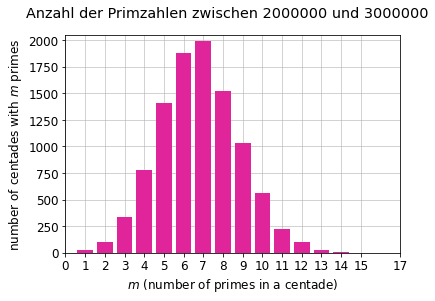
What proportion of centades between \(2\) and \(3\) million have exactly \(7\) primes, for instance? For such questions we can only conjecture an answer, for they seem to be well beyond current methods at present. Harald Cramér, a Swedish mathematician, statistician, and actuary, put forward a random model for the primes, that has led to many very fascinating and deep conjectures about the distribution of prime numbers. Cramér’s model gives us a conjectural answer to our question about the distribution of primes in intervals.
Let’s say we are looking at primes in intervals of the form \((a, a + H]\), for \(N - M < a \le N + M\), where \(N\) is very large and \(M\) is relatively small. By Gauss’s observation, confirmed by the prime number theorem, the density of primes around \(a\) is well-approximated by \(1/\log a\), which, since \(a\) is very close to \(N\), is well-approximated by \(1/\log N\). Cramér interpreted this density as a probability. Thus, what we ask for is the probability that the interval \((a, a + H]\) contains exactly \(m\) primes, when the probability that an integer chosen at random from the range in which the interval lies is prime, is close to \(1/\log N\). If we think of the indicator function of the primes in \((a, a + H]\) as the outcome of a sequence of \(H\) independent Bernoulli trials, with probability of a successful trial (the integer is prime) as \(1/\log N\), then we should expect the probability of the interval containing \(m\) primes to be approximated by the probability of \(m\) successful, and \(H - m\) unsuccessful, Bernoulli trials, viz.
\[\binom{H}{m}\left(\frac{1}{\log N}\right)^{m}\left(1 - \frac{1}{\log N}\right)^{H - m}.\]
The setup we’re interested in here is when \(H\) is of order \(\log N\) (the average size of the gap between consecutive primes around \(N\)). Thus, if \(H = \lambda \log N\), say, with \(\lambda > 0\) constant, the above can be written as
\[\binom{H}{m}\left(\frac{\lambda}{H}\right)^{m}\left(1 - \frac{\lambda}{H}\right)^{H - m},\]
which, by the Poisson limit theorem, is asymptotically equal to
\[\frac{e^{-\lambda}\lambda^m}{m!}\]
as \(N \to \infty\).
Now, there is a glaring problem with this heuristic, and that is related to the word independent. The event of an integer \(n\) being prime is certainly not independent of the event that \(n + 1\) is prime, for instance. (If \(n > 2\) is prime then it is odd and so \(n + 1\), being even, is certainly not prime.) Well, the Hardy-Littlewood prime \(k\)-tuples conjecture asserts, roughly speaking and continuing in our probabilistic vein, that the probability of a \(k\)-tuple \(n + h_1,\ldots, n + h_k\) of integers all being prime is close to
\[\frac{\mathfrak{S}(h_1,\ldots,h_k)}{(\log N)^k},\]
if \(n\) is very close to \(N\). Here \(\mathfrak{S}(h_1,\ldots,h_k)\) is a certain function of \(h_1,\ldots,h_k\), called the singular series for the \(k\)-tuple. Too our point about non-independence, \(\mathfrak{S}(0,1) = 0\), and \(\mathfrak{S}(h_1,\ldots,h_k) = 0\) whenever there is no chance of \(n + h_1,\ldots,n + h_k\) all being prime. (As another example, \(\mathfrak{S}(0,2,4) = 0\), because one of the integers \(n, n + 2, n + 4\) is always a multiple of \(3\).)
The naive application of Cramér’s model, which assumes independence, is basically asserting that the singular series is always equal to \(1\), which is wrong. However, it turns out that the singular series is very close to \(1\) on average, in the sense that
\[\sum_{0 < h_1 < \cdots < h_k \le H} \mathfrak{S}(h_1,\ldots,h_k) \sim \sum_{0 < h_1 < \cdots < h_k \le H} 1 \quad (H \to \infty).\]
This turns out to be enough to allow us to conclude, conditionally on a certain form of the Hardy-Littlewood prime \(k\)-tuples conjecture, that
\[\frac{1}{N} \#\{ a \le N : \pi(a + H) - \pi(a) = m \} \sim \frac{e^{-\lambda}\lambda^m}{m!} \quad (N \to \infty),\]
where \(\lambda > 0\) and \(m \ge 0\) are fixed, and where \(H = \lambda \log N\). This vindicates Cramér’s model: primes are distributed in short intervals essentially as if according to a Poisson process.
The result about the singular series, and the deduction of the conditional Poisson distribution for primes in short intervals, is due to Gallagher (Gallagher 1976), who used the method of moments. In (Freiberg 2018) we prove a generalization of this conditional result, using not the method of moments, but an inclusion-exclusion argument, that allows us to directly insert the sum over the singular series into the estimation of the probability mass function. Thus, we are able to make use of more precise estimates for the singular series average, such as the one due to Montgomery and Soundararajan (Montgomery and Soundararajan 2004), leading to more precise predictions with secondary terms (although we need to make further conjectures about the uniformity of the estimate of Montgomery and Soundararajan, or perhaps establish some unconditional results involving further averaging).
The resulting predictions for the distribution of primes in short intervals, agree with that of Cramér’s model (and the conditional result of Gallagher) as first-order approximations, but deviate at the second-order term, and appear to better fit the numerical data, where it seems the expected number of primes in an interval is much more popular of a value than is suggested by Cramér’s model. The purpose of the code in this project is to generate data for primes in intervals, compare it to theoretical predictions, and visualize the results in tables and plots.