This is the entry point. It establishes what the dataset contains, what is awkward about it, and which of those awkward properties drive design decisions later in the project.
Three findings here shape everything downstream:
The dataset is severely imbalanced, so plain accuracy is not a usable metric.
Many lesions are photographed more than once, so an image-level train/test split would leak.
How often a lesion was photographed is itself informative about its diagnosis, which makes it a tempting and dangerous feature, and makes the choice of one-image-per-lesion versus all-images a question about the training distribution rather than about data volume.
2.1 The dataset
HAM10000 (“Human Against Machine with 10000 training images”) is 10,015 dermatoscopic images collected across several populations and imaging modalities, released by Tschandl, Rosendahl and Kittler (2018). Seven diagnostic classes:
Code
Diagnosis
Malignant
akiec
Actinic keratoses / intraepithelial carcinoma
pre-malignant
bcc
Basal cell carcinoma
yes
bkl
Benign keratosis-like lesions
no
df
Dermatofibroma
no
mel
Melanoma
yes
nv
Melanocytic nevi (moles)
no
vasc
Vascular lesions
no
Ground truth comes from histopathology for a little over half the cases; the rest from follow-up examination, expert consensus, or confocal microscopy. That distinction matters more than it first appears; see the section on multiplicity.
Caveat.Wen et al. (2022) note that public dermatoscopic datasets, HAM10000 included, report little about ethnicity or Fitzpatrick skin type, and that classifiers trained on one population routinely underperform on another. Nothing in this project addresses that. Any model trained here should be understood as fitted to the populations these images came from, which are not documented well enough to characterise.
2.2 Setup
Code
from pathlib import Pathimport pandas as pdfrom ham10000.config import Settingsfrom ham10000.data import load_metadatafrom ham10000.exploration import frequenciessettings = Settings.resolve()metadata = load_metadata(settings.metadata_csv)print(f"{len(metadata):,} images of {metadata['lesion_id'].nunique():,} lesions")metadata.head()
10,015 images of 7,470 lesions
lesion_id
num_images
image_id
dx
dx_type
age
sex
localization
0
HAM_0000118
2
ISIC_0027419
bkl
histo
80.0
male
scalp
1
HAM_0000118
2
ISIC_0025030
bkl
histo
80.0
male
scalp
2
HAM_0002730
2
ISIC_0026769
bkl
histo
80.0
male
scalp
3
HAM_0002730
2
ISIC_0025661
bkl
histo
80.0
male
scalp
4
HAM_0001466
2
ISIC_0031633
bkl
histo
75.0
male
ear
2.3 Class imbalance
The first thing to establish, because it determines how the model is evaluated.
Table 2.1: Class distribution over distinct lesions.
dx
nv
bkl
mel
bcc
akiec
vasc
df
freq
5403.00
727.00
614.00
327.00
228.00
98.00
73.00
%
72.33
9.73
8.22
4.38
3.05
1.31
0.98
Nevi are over 72% of lesions and dermatofibroma under 1%. That share is counted over lesions rather than images, because a lesion is the unit everything here is scored on: one photographed five times is one case, not five.
A classifier that answers “nevus” every time therefore scores ~72% plain accuracy while being clinically worthless.
This is why balanced accuracy is the headline metric throughout this project. It is the mean of per-class recall, and recall for class c is P(predict c | true class is c). If a rule ignores the image, its prediction is independent of the truth, so that conditioning does nothing: recall for each class is simply how often the rule happens to say that class. Those frequencies sum to 1 across the n classes, so their mean is 1/n whatever the rule, and however imbalanced the data.
The floor is therefore 1/7 = 0.143 for any strategy that does not look at the image. The always-nevus classifier is just one such strategy:
Rule
Plain accuracy
Balanced accuracy
uniform random
0.143
0.142
random, weighted by class frequency
0.543
0.144
always nevus
0.723
0.143
always dermatofibroma
0.010
0.143
Plain accuracy varies 70-fold across those four; balanced accuracy does not move. Beating 0.143, then, is evidence that a model is reading the image, which is exactly what plain accuracy fails to tell us.
These baselines are computed on this dataset’s class distribution. The balanced-accuracy floor of 1/n does not depend on it (the derivation never uses the class frequencies), but the plain-accuracy figures do, and would change on a population with different prevalence. The split is stratified, so training and validation proportions agree to within 0.1 points; balancing then deliberately makes the training distribution uniform, which is why a metric insensitive to the prior is the right one.
How exactly are these baseline metrics computed? With n classes, write q_c for the fraction of cases whose true class is c, and recall_c for the fraction of class-c cases the classifier gets right. Both metrics are weighted averages of the same per-class recalls, differing only in the weights:
Plain accuracy weights each class by how often it occurs; balanced accuracy weights every class equally. That is why one is fooled by imbalance and the other is not.
Now take a classifier that ignores the image, saying class c with probability p_c. Independence makes the conditioning in recall vacuous, so recall_c = p_c, and:
The class distribution has vanished from the second: no input-blind rule can beat 1/n, whatever it predicts. Plain accuracy still contains q, and can be inflated by aligning p with it, which is exactly what “always nevus” does.
2.4 Lesion multiplicity, and why the split happens at the lesion level
Many lesions were photographed more than once. Those images are near-duplicates of each other.
Table 2.2: Number of lesions by how many times each was photographed.
num_images
1
2
3
4
5
6
lesions
5514
1423
490
34
5
4
Code
repeated =int((lesions["num_images"] >1).sum())print(f"{repeated:,} lesions have more than one image "f"({repeated /len(lesions):.1%} of lesions)")
1,956 lesions have more than one image (26.2% of lesions)
An image-level train/test split would place near-identical photographs of the same lesion on both sides of the boundary. The resulting validation score would measure memorisation, not generalisation. ham10000.data.splitting therefore assigns every image of a lesion to the same side. The guarantee is checkable rather than merely claimed:
Code
from ham10000.data import SplitConfig, assign_splits, lesion_overlapfrom ham10000.data import LabelSchemescheme = LabelScheme.build(sorted(metadata["dx"].unique()), set(metadata["dx"].unique()))metadata["label"] = metadata["dx"].map(scheme.mapping)assignment = assign_splits(metadata, SplitConfig(seed=0))annotated = metadata.assign(set=assignment.sets)print("lesions appearing on both sides:", lesion_overlap(annotated) or"none")print(f"train lesions: {len(assignment.train_lesions):,}")print(f"val lesions: {len(assignment.val_lesions):,}")
lesions appearing on both sides: none
train lesions: 5,600
val lesions:   1,870
2.5 Multiplicity is not random
This is the least obvious property of the dataset, and it has consequences. A physician takes one dermatoscopic image of a lesion they are confident about. They take several, and then a biopsy, when they are not. So the number of images of a lesion records how uncertain its diagnosis was, and uncertainty is not independent of what the lesion turned out to be.
Table 2.3: How nevi were diagnosed, by the number of images of the lesion (%).
dx_type
consensus
follow_up
histo
num_images
1
4.1
83.9
12.0
2
19.2
0.0
80.8
3
4.1
0.0
95.9
4
11.1
0.0
88.9
5
50.0
0.0
50.0
6
100.0
0.0
0.0
The discontinuity is near-total (Table 2.3). A nevus photographed once was usually confirmed by follow-up; a nevus photographed twice or more was almost never confirmed by follow-up and almost always by histopathology. Multiplicity is effectively a record of whether the clinician was worried enough to biopsy. The same signal appears across classes:
Table 2.4: Mean number of images per lesion, by diagnosis.
mean
count
dx
nv
1.24
5403
akiec
1.43
228
vasc
1.45
98
bkl
1.51
727
bcc
1.57
327
df
1.58
73
mel
1.81
614
Melanoma is the most-photographed class and nevus the least (Table 2.4).
Two consequences:
num_images must never be used as a feature. It is a proxy for clinical concern, which is downstream of the label. A model given it would score well and have learned nothing about skin.
Choosing one image per lesion versus all images is not a question about data volume. Training on all images oversamples exactly the lesions that were photographed repeatedly: the ambiguous ones, and disproportionately the malignant ones. It changes both the class prior and the difficulty distribution of the training set. Both settings are supported in configs/, and the difference between them should be read in this light rather than as “more data versus less”.
The same signal read the other way round. Instead of asking how a lesion was diagnosed given how often it was photographed, ask what it turned out to be.
Table 2.5: Diagnosis given the number of images of a lesion (%).
num_images
1
2
3
4
5
6
dx
akiec
2.74
4.01
3.67
5.88
0.0
0.0
bcc
3.17
8.29
6.73
2.94
0.0
0.0
bkl
7.98
15.46
11.22
23.53
40.0
50.0
df
0.71
1.83
1.63
0.00
0.0
0.0
mel
4.17
19.54
20.41
11.76
20.0
25.0
nv
80.07
49.12
54.69
52.94
40.0
25.0
vasc
1.16
1.76
1.63
2.94
0.0
0.0
Melanoma is 4.2% of lesions photographed once (Table 2.5), and roughly 20% of those photographed two or three times. Conditioning on a second photograph nearly quintuples the melanoma rate. Nevi move the other way, from 80% down to about half.
The same effect shows up a third time, in how the diagnoses were confirmed. Follow-up examination accounts for 49.6% of lesions but only 37.0% of images, while histopathology accounts for 41.3% of lesions and 53.3% of images. Biopsied lesions were photographed more often, which is the same fact stated in terms of images rather than lesions.
Table 2.6: How diagnoses were confirmed, counted over lesions and over images.
lesions %
images %
dx_type
confocal
0.46
0.69
consensus
8.66
9.01
follow_up
49.59
36.98
histo
41.30
53.32
Atypical nevi
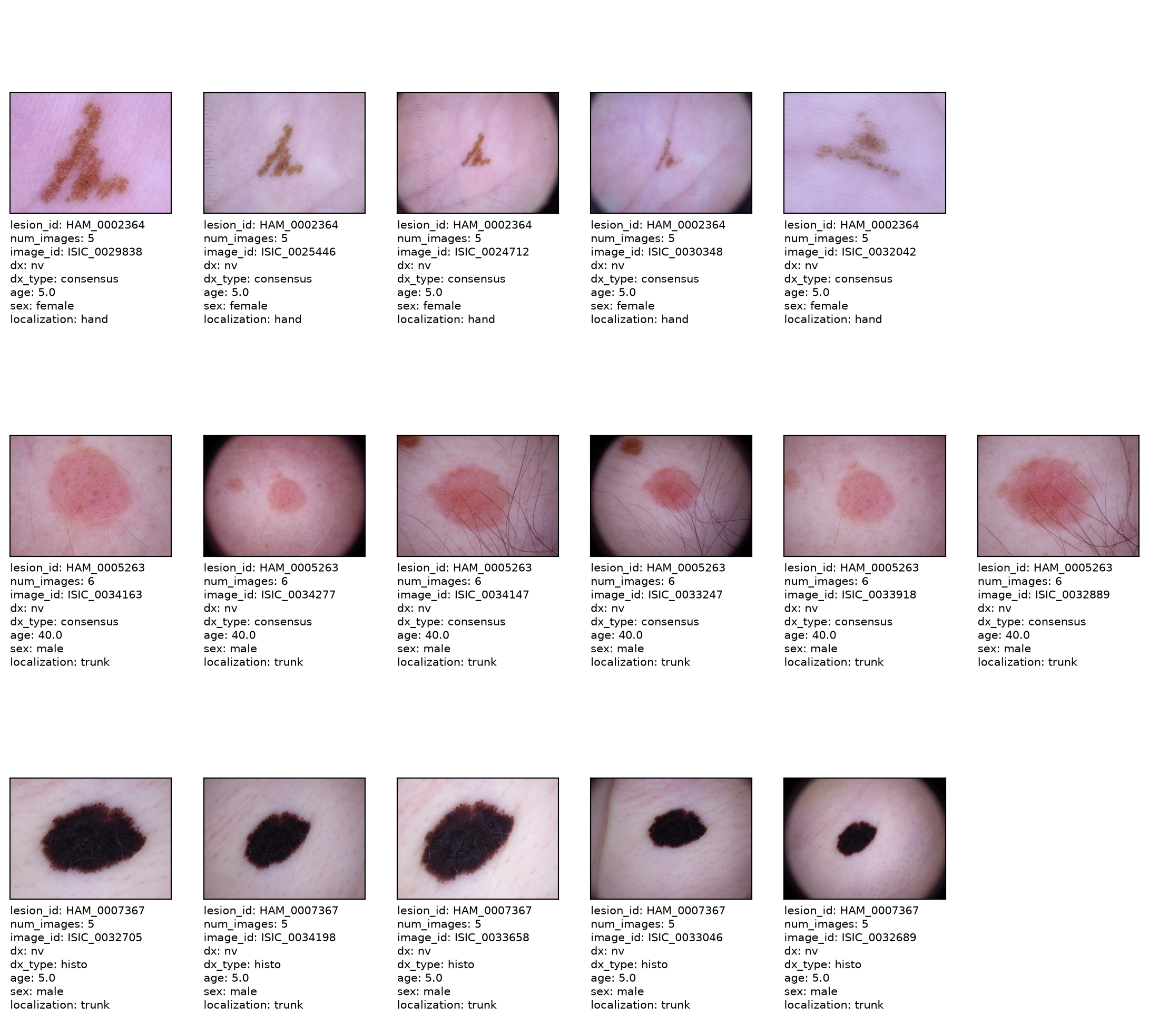
Three nevi were photographed five or six times, more than any other lesion in the dataset. Worth looking at, because it is easy to see why the clinician kept going. They are genuinely odd: irregular in outline, unevenly pigmented, the sort of thing the ABCD rule would flag.
One was biopsied and two were settled by expert consensus, and all three came back benign. That is the useful part. An atypical lesion is not a melanoma, it is a lesion someone had to work to rule out, and these are what that looks like. Two of the three belong to five-year-olds, where an unusual-looking mole is common and melanoma is vanishingly rare.
Figure 2.1: The three nevi photographed five or six times. All benign.
2.6 Artefacts
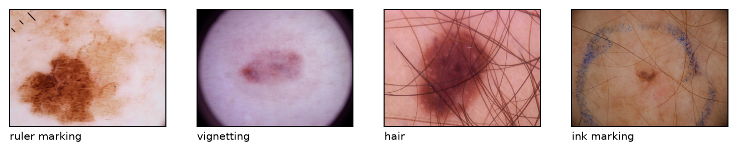
Dermatoscopic images contain things that are not the lesion (Figure 2.2): ink markings where a physician outlined it, ruler markings, hair, and dark vignetting from the dermatoscope aperture. Some of these are present by design: in the manual quality review described by Tschandl, Rosendahl, and Kittler (2018), images with obstructing gel bubbles were excluded, while terminal hairs were specifically tolerated.
Artefacts matter if they correlate with diagnosis, and there is reason to think some do. A lesion a physician bothered to mark and measure is a lesion they were concerned about, which is the same mechanism that makes multiplicity informative. This is not speculation: Winkler et al. (2019) examined the association between surgical skin markings and a melanoma classifier’s diagnostic performance, and a companion study (Winkler et al. 2021) did the same for scale bars in images shown to a market-approved network. Katsch, Rinner, and Tschandl (2022) tested robustness on HAM10000 itself by superimposing artefact templates, and found a decrease in area under the precision-recall curve of 0.030 for ResNet-34 and 0.045 for Faster R-CNN against 0.011 for Mask R-CNN, with the important detail that the effect only became significant once 40% or more of images carried artefacts, and that performance loss also occurred when artefacts were selectively superimposed on one class during training.
That last point is the one that bears on this project: the risk is not artefacts as such, but artefacts distributed unevenly across classes. Nothing here removes them or measures their distribution.
A separate problem is not what the image contains but what it leaves out. Polarised and non-polarised dermatoscopy show different features, and some of the features that matter most appear in only one mode. Shiny white lines, visible under polarised light and not otherwise, carry an odds ratio of 6.7 for melanoma in meta-analysis, equal to the highest of any dermatoscopic feature. They are also angle-dependent, so the instrument has to be rotated to bring them out. Whybrew et al. (2022) photographed one pigmented lesion with six different dermatoscopes and two cameras, rotating each to obtain the strongest display they could: five instruments showed the lines, and the sixth, a Heine DELTA 30, did not, its polarised images being essentially identical to its non-polarised ones. The lesion was a superficial spreading melanoma in situ.
This matters for a dataset assembled over twenty years from two clinical sites. HAM10000 records no instrument, no imaging mode and no acquisition angle. So an image lacking a top-odds-ratio feature may be an image of a lesion without it, or an image taken in the wrong mode, or an image taken on a device that does not render it. Nothing in the metadata distinguishes those cases, and no amount of training data recovers a feature that was never captured.
The crops discard information too. Polarising-specific white lines also occur on severely sun-damaged skin, so whether their presence in a lesion means anything depends on whether the surrounding skin shows them as well: Rosendahl and Marozava (2019) advises always looking at the skin beside the lesion when evaluating any structure. The same applies to the “ugly duckling” sign, where what marks a lesion as suspicious is that it looks unlike the person’s other lesions. A tightly cropped image supports neither comparison.
dx is constant for every lesion, which the whole project depends on: the label is a property of the lesion, not of the photograph. localization is not always constant. The affected lesions are recorded as e.g. ‘chest’, ‘chest’, ‘trunk’. The categories are not mutually exclusive and not uniformly specific, since the chest is part of the trunk. This is a limitation of the annotation scheme rather than an error in the data, and it means localization should be treated as coarse if used at all.
2.8 Missing values
Code
# `age` records missing values as NaN, but `sex` and `localization` use the# string "unknown". `isna()` sees only the first kind, so count both.absent_age = per_lesion_missing = lesions["age"].isna()absent_sex = lesions["sex"] =="unknown"absent_site = lesions["localization"] =="unknown"pd.Series( {"age": int(absent_age.sum()),"sex": int(absent_sex.sum()),"localization": int(absent_site.sum()),"at least one of the three": int((absent_age | absent_sex | absent_site).sum()),"all three": int((absent_age & absent_sex & absent_site).sum()), }, name="distinct lesions affected",).to_frame()
Table 2.7: Lesions with missing age, sex or body site.
distinct lesions affected
age
52
sex
50
localization
203
at least one of the three
213
all three
46
Missingness is recorded two different ways. Age uses NaN, while sex and body site use the string unknown, so isna() alone undercounts it and reports only the 52 lesions with no age. Counting both, 213 lesions (2.85%) are missing at least one of the three, and 46 are missing all three. Body site is the most often absent, at 203 lesions.
2.9 Do the other features carry signal?
The dataset records age, sex and body site alongside each lesion. None of the models in this project use them, since the classifiers work from pixels alone. It is still worth asking whether they would have helped.
The test below fits a gradient-boosted tree on those three columns only, with no access to the image. It uses the same lesion-level split as everything else, so the model never sees a validation lesion during training. Sex and body site are encoded as integer categories, which is why unknown simply becomes one more category rather than needing to be imputed. Classes are weighted by inverse frequency during fitting, for the same reason balancing exists in the image pipeline: without it the model would answer nevus every time. The score is balanced accuracy on validation lesions, so it is directly comparable with the image models.
That is well above chance, so the features are not noise. It is also well below what the image models reach. The more interesting question is which classes the signal belongs to.
Code
recalls = recall_score( validation["target"], predicted, average=None, zero_division=0)pd.Series( {scheme.codes[i]: round(r, 3) for i, r inenumerate(recalls)}, name="recall from metadata alone",).sort_values(ascending=False).to_frame()
Table 2.8: Per-class recall from age, sex and body site alone.
recall from metadata alone
df
0.579
akiec
0.491
nv
0.365
bcc
0.305
vasc
0.200
mel
0.162
bkl
0.132
Dermatofibroma and actinic keratosis are the classes it predicts best (Table 2.8), which makes sense: actinic keratosis is sun-damaged skin on the face and scalp of older patients, and dermatofibroma sits on the limbs. Both are close to being defined by where they appear and who they appear on.
Melanoma comes last of the seven. The demographic features are informative about the classes that matter least, and close to useless for the one that matters most. So the answer is that these features carry real signal, and that using them would be unlikely to help with the decision this project cares about. Combining tabular features with pixels in one model is a worthwhile exercise, but it is a different project.
Katsch, Florian, Christoph Rinner, and Philipp Tschandl. 2022. “Comparison of Convolutional Neural Network Architectures for Robustness Against Common Artefacts in Dermatoscopic Images.”Dermatology Practical & Conceptual 12 (3): e2022126. https://doi.org/10.5826/dpc.1203a126.
Rosendahl, Cliff, and Aksana Marozava. 2019. Dermatoscopy and Skin Cancer: A Handbook for Hunters of Skin Cancer and Melanoma. First. Banbury, UK: Scion Publishing Ltd.
Tschandl, Philipp, Cliff Rosendahl, and Harald Kittler. 2018. “The HAM10000 Dataset, a Large Collection of Multi-Source Dermatoscopic Images of Common Pigmented Skin Lesions.”Scientific Data 5: 180161. https://doi.org/10.1038/sdata.2018.161.
Wen, David, Saad M. Khan, Antonio Ji Xu, Hussein Ibrahim, Luke Smith, Jose Caballero, Luis Zepeda, et al. 2022. “Characteristics of Publicly Available Skin Cancer Image Datasets: A Systematic Review.”The Lancet Digital Health 4 (1): e64–74. https://doi.org/10.1016/S2589-7500(21)00252-1.
Whybrew, Chin, Paweł Pietkiewicz, Ihor Kohut, Justin C. Chia, Bengu Nisa Akay, and Cliff Rosendahl. 2022. “Not All Polarized-Light Dermatoscopes May Display Diagnostically Critical Polarizing-Specific Features.”Dermatology Practical & Conceptual 12 (4): e2022250. https://doi.org/10.5826/dpc.1204a250.
Winkler, Julia K., Christine Fink, Ferdinand Toberer, Alexander Enk, Teresa Deinlein, Rainer Hofmann-Wellenhof, Luc Thomas, et al. 2019. “Association Between Surgical Skin Markings in Dermoscopic Images and Diagnostic Performance of a Deep Learning Convolutional Neural Network for Melanoma Recognition.”JAMA Dermatology 155 (10): 1135–41. https://doi.org/10.1001/jamadermatol.2019.1735.
Winkler, Julia K., Katharina Sies, Christine Fink, Ferdinand Toberer, Alexander Enk, Andreas Blum, Wilhelm Stolz, Albert Rosenberger, and Holger A. Haenssle. 2021. “Association Between Different Scale Bars in Dermoscopic Images and Diagnostic Performance of a Market-Approved Deep Learning Convolutional Neural Network for Melanoma Recognition.”European Journal of Cancer 145: 146–54. https://doi.org/10.1016/j.ejca.2020.12.010.