An Analysis of Euclid’s Algorithm
1 Introduction
Euclid’s algorithm “might be called the grandaddy of all algorithms”, as Knuth aptly put it (Knuth 1997). Countless modern-day students know the joy of performing the algorithm by hand, essentially in the form set down by Euclid in his Elements over two thousand years ago. Analyses of the algorithm go back as far as the 18th century, when it was understood (at least implicitly) that consecutive Fibonacci numbers give rise to the worst-case in terms of the number of divisions performed, relative to the size of the inputs. Average-case analyses and finer points received surprisingly little attention until the latter half of the last century. (See Knuth (Knuth 1997) and Shallit (Shallit 1994) for superlatively detailed accounts of the algorithm’s fascinating history.) Only in recent decades has Euclid’s algorithm been put into a general framework for the analysis of algorithms (by Baladi and Vallée (Baladi and Vallée 2005) et al.), in which certain algorithms are viewed as dynamical systems: the mathematics is as beautiful as it is deep. Although the current state-of-the-art paints a fairly detailed picture with respect to the distributional analysis of Euclid’s algorithm, it still tantalises us with open questions, and these questions remain focal points of some exciting research programmes.
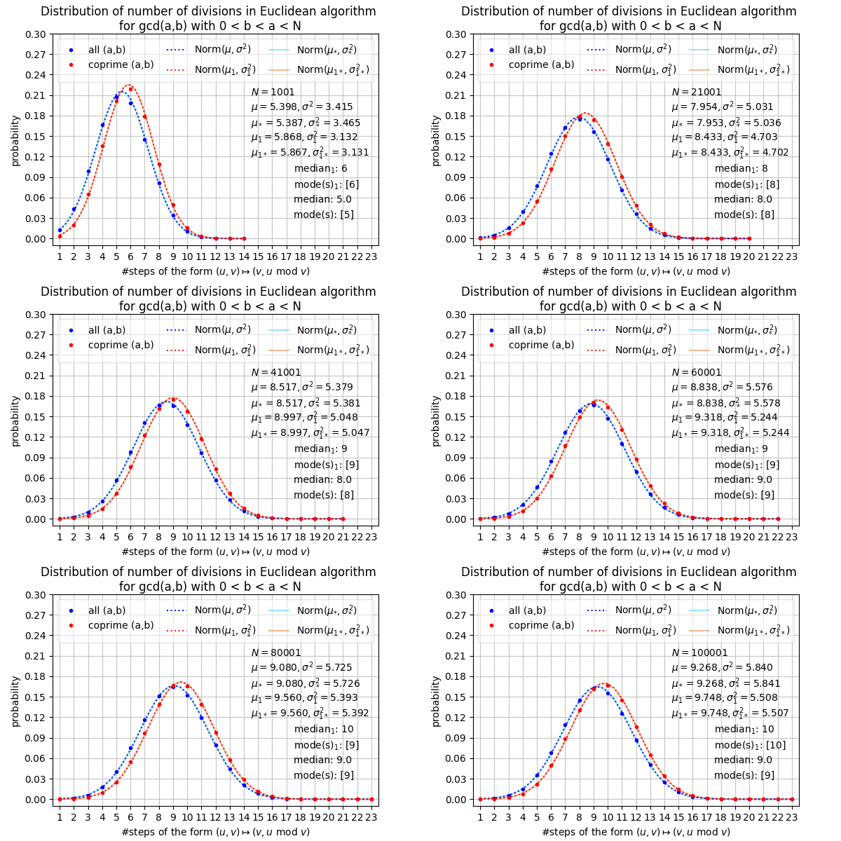
Indeed, one of our goals here is to shed some light (numerically) on a certain “obscure” constant that arises in the analysis of Euclid’s algorithm. Our main goal, though, is simply to demonstrate how fun and instructive it can be to study introductory discrete mathematics and statistics alongside basic Python. We’ll code Euclid’s algorithm, apply it to almost five billion pairs of integers to produce some data, then tabulate and visualise the results (the above animation is just one example). Along the way, we’ll discuss the Fibonacci numbers and touch on dynamic programming, among other things like random walks… Libraries we’ll use include NumPy, SciPy, Matplotlib, and pandas.
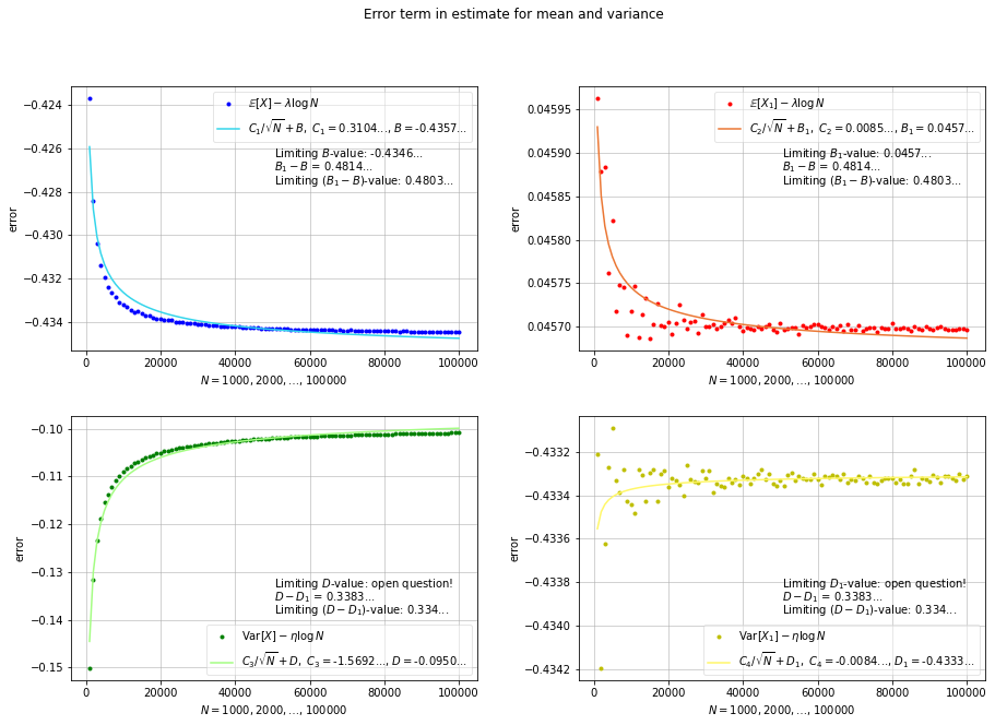
There are various ways of analysing Euclid’s algorithm. Here is one example. Let \(X\) be the random variable whose value is the number of divisions performed in the computation of \(\gcd(a,b)\) via Euclid’s algorithm, with \((a,b)\) chosen uniformly at random from the region \(1 \le b < a \le N\). It is known that \(X\) is asymptotically normal (as \(N \to \infty\)), with mean close to \(\lambda\log N + \nu - \frac{1}{2}\) and variance close to \(\eta\log N + \kappa\), for certain constants \(\lambda, \nu, \eta, \kappa\). While the constants associated with the mean can be written in closed form, and therefore calculated to any desired degree of accuracy with relative ease (\(\lambda = 0.8427659\ldots\) and \(\nu = 0.0653514\ldots\)), this is not so for the constants associated with the variance. Nevertheless, Lhote (Lhote 2005) showed that \(\eta\) is polynomial-time computable, and determined its first seven digits: \(\eta = 0.5160524\ldots\). The “subdominant” constant \(\kappa\) is even more mysterious, and our numerics will lead us to guess an approximate value for it (we believe it is around \(-0.1\)).
In the above animation, the distribution of \(X\) is shown for various \(N\) up to \(10^5\) (starting with \(N = 1000\) and going up by \(1000\) in each frame). The large blue dots give the probability that \(X\) equals a given number on the horizontal axis. The dotted blue curve is normal with mean \(\mu = \mathbb{E}[X]\) and variance \(\sigma^2 = \mathrm{Var}(X)\), while the light blue curve is normal with mean \(\mu_* = \lambda\log N + \nu - \frac{1}{2}\) and variance \(\sigma_*^2 = \eta \log N - 0.1\). The red dots and curves are analogous, but only coprime pairs \((a,b)\) are considered. See Two-dimensional analysis: distribution for more detail and context.
1.1 Some plots
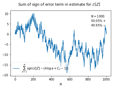
Is this a random walk? See One-dimensional analysis: mean and error term for the answer.
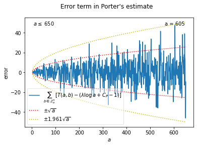
See One-dimensional analysis: mean and error term for the context of this instance of square-root-cancellation.
See One-dimensional analysis: variance for more about the next two plots.
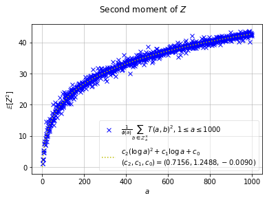
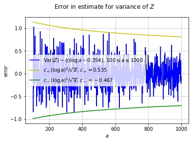
See One-dimensional analysis: distribution for an explanation of the animation below.
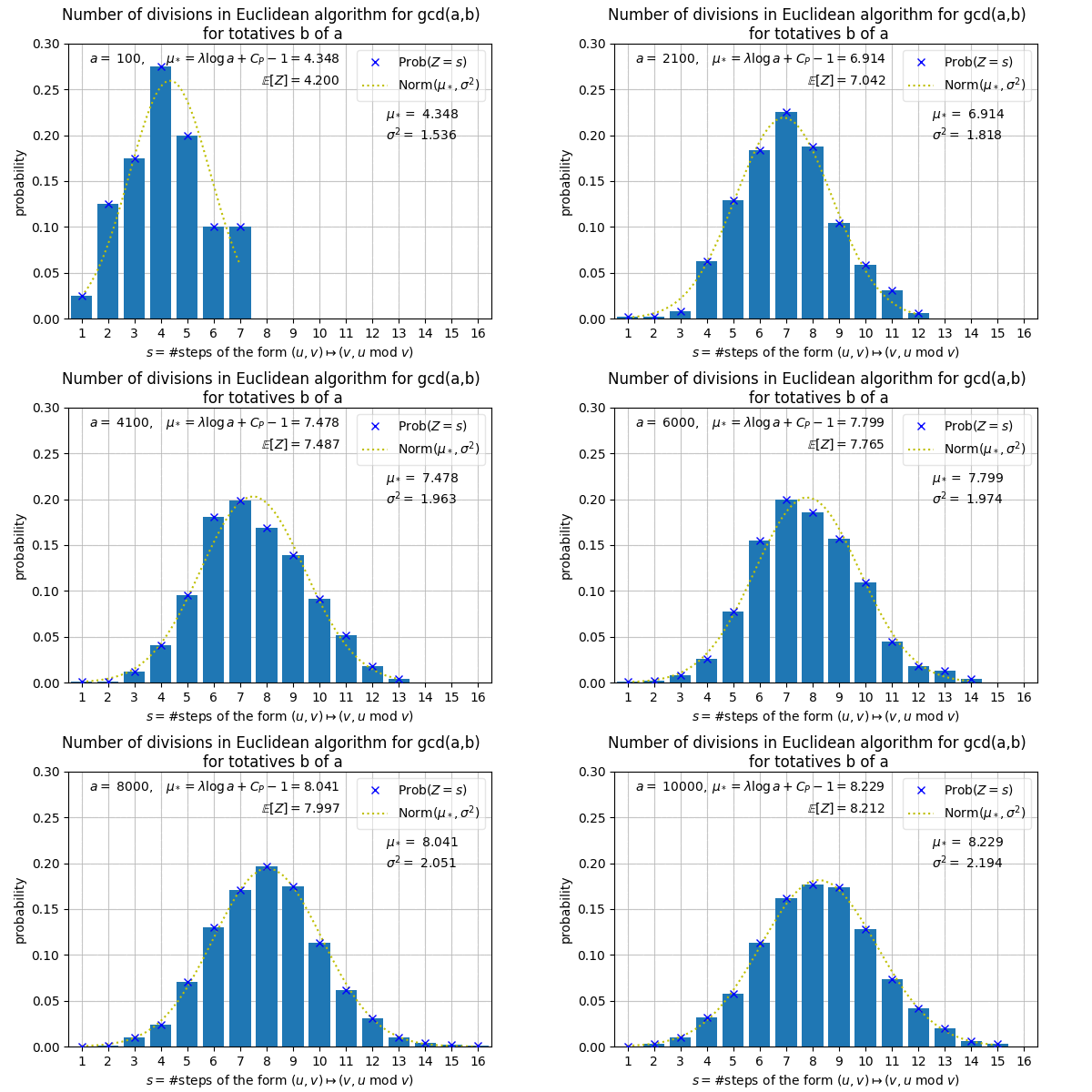
See Two-dimensional analysis: error terms & subdominant constant in the variance for an explanation of the plots below.